In physics, the cross section is a measure of the probability that a specific process will take place when some kind of radiant excitation intersects a localized phenomenon. For example, the Rutherford cross-section is a measure of probability that an alpha particle will be deflected by a given angle during an interaction with an atomic nucleus. Cross section is typically denoted σ (sigma) and is expressed in units of area, more specifically in barns. In a way, it can be thought of as the size of the object that the excitation must hit in order for the process to occur, but more exactly, it is a parameter of a stochastic process.

In mathematical analysis, the Dirac delta distribution, also known as the unit impulse, is a generalized function or distribution over the real numbers, whose value is zero everywhere except at zero, and whose integral over the entire real line is equal to one.
A Fourier series is an expansion of a periodic function into a sum of trigonometric functions. The Fourier series is an example of a trigonometric series, but not all trigonometric series are Fourier series. By expressing a function as a sum of sines and cosines, many problems involving the function become easier to analyze because trigonometric functions are well understood. For example, Fourier series were first used by Joseph Fourier to find solutions to the heat equation. This application is possible because the derivatives of trigonometric functions fall into simple patterns. Fourier series cannot be used to approximate arbitrary functions, because most functions have infinitely many terms in their Fourier series, and the series do not always converge. Well-behaved functions, for example smooth functions, have Fourier series that converge to the original function. The coefficients of the Fourier series are determined by integrals of the function multiplied by trigonometric functions, described in Common forms of the Fourier series below.

In mathematics and physics, the heat equation is a certain partial differential equation. Solutions of the heat equation are sometimes known as caloric functions. The theory of the heat equation was first developed by Joseph Fourier in 1822 for the purpose of modeling how a quantity such as heat diffuses through a given region.
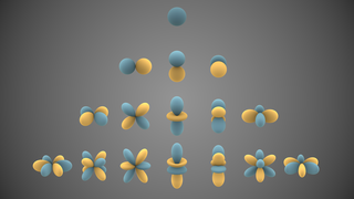
In mathematics and physical science, spherical harmonics are special functions defined on the surface of a sphere. They are often employed in solving partial differential equations in many scientific fields. A list of the spherical harmonics is available in Table of spherical harmonics.
In mathematics, a Gaussian function, often simply referred to as a Gaussian, is a function of the base form
In mathematics, the Fourier inversion theorem says that for many types of functions it is possible to recover a function from its Fourier transform. Intuitively it may be viewed as the statement that if we know all frequency and phase information about a wave then we may reconstruct the original wave precisely.
In mathematics and signal processing, the Hilbert transform is a specific singular integral that takes a function, u(t) of a real variable and produces another function of a real variable H(u)(t). The Hilbert transform is given by the Cauchy principal value of the convolution with the function (see § Definition). The Hilbert transform has a particularly simple representation in the frequency domain: It imparts a phase shift of ±90° (π/2 radians) to every frequency component of a function, the sign of the shift depending on the sign of the frequency (see § Relationship with the Fourier transform). The Hilbert transform is important in signal processing, where it is a component of the analytic representation of a real-valued signal u(t). The Hilbert transform was first introduced by David Hilbert in this setting, to solve a special case of the Riemann–Hilbert problem for analytic functions.
In the theory of stochastic processes, the Karhunen–Loève theorem, also known as the Kosambi–Karhunen–Loève theorem states that a stochastic process can be represented as an infinite linear combination of orthogonal functions, analogous to a Fourier series representation of a function on a bounded interval. The transformation is also known as Hotelling transform and eigenvector transform, and is closely related to principal component analysis (PCA) technique widely used in image processing and in data analysis in many fields.

In system analysis, among other fields of study, a linear time-invariant (LTI) system is a system that produces an output signal from any input signal subject to the constraints of linearity and time-invariance; these terms are briefly defined below. These properties apply (exactly or approximately) to many important physical systems, in which case the response y(t) of the system to an arbitrary input x(t) can be found directly using convolution: y(t) = (x ∗ h)(t) where h(t) is called the system's impulse response and ∗ represents convolution (not to be confused with multiplication). What's more, there are systematic methods for solving any such system (determining h(t)), whereas systems not meeting both properties are generally more difficult (or impossible) to solve analytically. A good example of an LTI system is any electrical circuit consisting of resistors, capacitors, inductors and linear amplifiers.
In mathematics, a fundamental solution for a linear partial differential operator L is a formulation in the language of distribution theory of the older idea of a Green's function.
In mathematics, and specifically in potential theory, the Poisson kernel is an integral kernel, used for solving the two-dimensional Laplace equation, given Dirichlet boundary conditions on the unit disk. The kernel can be understood as the derivative of the Green's function for the Laplace equation. It is named for Siméon Poisson.
In probability theory, calculation of the sum of normally distributed random variables is an instance of the arithmetic of random variables.
In mathematics, the secondary measure associated with a measure of positive density ρ when there is one, is a measure of positive density μ, turning the secondary polynomials associated with the orthogonal polynomials for ρ into an orthogonal system.

Photon transport in biological tissue can be equivalently modeled numerically with Monte Carlo simulations or analytically by the radiative transfer equation (RTE). However, the RTE is difficult to solve without introducing approximations. A common approximation summarized here is the diffusion approximation. Overall, solutions to the diffusion equation for photon transport are more computationally efficient, but less accurate than Monte Carlo simulations.
In mathematics, vector spherical harmonics (VSH) are an extension of the scalar spherical harmonics for use with vector fields. The components of the VSH are complex-valued functions expressed in the spherical coordinate basis vectors.
Common integrals in quantum field theory are all variations and generalizations of Gaussian integrals to the complex plane and to multiple dimensions. Other integrals can be approximated by versions of the Gaussian integral. Fourier integrals are also considered.
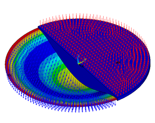
Bending of plates, or plate bending, refers to the deflection of a plate perpendicular to the plane of the plate under the action of external forces and moments. The amount of deflection can be determined by solving the differential equations of an appropriate plate theory. The stresses in the plate can be calculated from these deflections. Once the stresses are known, failure theories can be used to determine whether a plate will fail under a given load.
Filtering in the context of large eddy simulation (LES) is a mathematical operation intended to remove a range of small scales from the solution to the Navier-Stokes equations. Because the principal difficulty in simulating turbulent flows comes from the wide range of length and time scales, this operation makes turbulent flow simulation cheaper by reducing the range of scales that must be resolved. The LES filter operation is low-pass, meaning it filters out the scales associated with high frequencies.
In mathematics, singular integral operators of convolution type are the singular integral operators that arise on Rn and Tn through convolution by distributions; equivalently they are the singular integral operators that commute with translations. The classical examples in harmonic analysis are the harmonic conjugation operator on the circle, the Hilbert transform on the circle and the real line, the Beurling transform in the complex plane and the Riesz transforms in Euclidean space. The continuity of these operators on L2 is evident because the Fourier transform converts them into multiplication operators. Continuity on Lp spaces was first established by Marcel Riesz. The classical techniques include the use of Poisson integrals, interpolation theory and the Hardy–Littlewood maximal function. For more general operators, fundamental new techniques, introduced by Alberto Calderón and Antoni Zygmund in 1952, were developed by a number of authors to give general criteria for continuity on Lp spaces. This article explains the theory for the classical operators and sketches the subsequent general theory.


