Monochrome light beam whose amplitude envelope is a Gaussian function
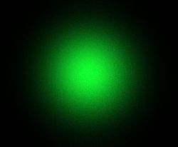
Instantaneous absolute value of the real part of electric field amplitude of a TEM00 Gaussian beam, focal region. Showing thus with two peaks for each positive wavefront.Top: transverse intensity profile of a Gaussian beam that is propagating out of the page. Blue curve: electric (or magnetic) field amplitude vs. radial position from the beam axis. The black curve is the corresponding intensity.A 5 mW green laser pointer beam, showing the TEM00 profile
In optics, a Gaussian beam is an idealized beam of electromagnetic radiation whose amplitude envelope in the transverse plane is given by a Gaussian function; this also implies a Gaussian intensity (irradiance) profile. This fundamental (or TEM00) transverse Gaussian mode describes the intended output of many lasers, as such a beam diverges less and can be focused better than any other. When a Gaussian beam is refocused by an ideal lens, a new Gaussian beam is produced. The electric and magnetic field amplitude profiles along a circular Gaussian beam of a given wavelength and polarization are determined by two parameters: the waistw0, which is a measure of the width of the beam at its narrowest point, and the position z relative to the waist.[1]
Since the Gaussian function is infinite in extent, perfect Gaussian beams do not exist in nature, and the edges of any such beam would be cut off by any finite lens or mirror. However, the Gaussian is a useful approximation to a real-world beam for cases where lenses or mirrors in the beam are significantly larger than the spot size w(z) of the beam.
Fundamentally, the Gaussian is a solution of the paraxial Helmholtz equation, the wave equation for an electromagnetic field. Although there exist other solutions, the Gaussian families of solutions are useful for problems involving compact beams.
Mathematical form
The equations below assume a beam with a circular cross-section at all values of z; this can be seen by noting that a single transverse dimension, r, appears. Beams with elliptical cross-sections, or with waists at different positions in z for the two transverse dimensions (astigmatic beams) can also be described as Gaussian beams, but with distinct values of w0 and of the z = 0 location for the two transverse dimensions x and y.
Gaussian beam intensity profile with w0 = 2λ.
The Gaussian beam is a transverse electromagnetic (TEM) mode.[2] The mathematical expression for the electric field amplitude is a solution to the paraxial Helmholtz equation.[1] Assuming polarization in the x direction and propagation in the +z direction, the electric field in phasor (complex) notation is given by:
k = 2πn/λ is the wave number (in radians per meter) for a free-space wavelength λ, and n is the index of refraction of the medium in which the beam propagates,
E0 = E(0, 0), the electric field amplitude at the origin (r = 0, z = 0),
w(z) is the radius at which the field amplitudes fall to 1/e of their axial values (i.e., where the intensity values fall to 1/e2 of their axial values), at the plane z along the beam,
Since this solution relies on the paraxial approximation, it is not accurate for very strongly diverging beams. The above form is valid in most practical cases, where w0 ≫ λ/n.
where the constant η is the wave impedance of the medium in which the beam is propagating. For free space, η = η0 ≈ 377 Ω. I0 = |E0|2/2η is the intensity at the center of the beam at its waist.
The Gaussian function has a 1/e diameter (2w as used in the text) about 1.7 times the FWHM.
At a position z along the beam (measured from the focus), the spot size parameter w is given by a hyperbolic relation:[1] where[1] is called the Rayleigh range as further discussed below, and is the refractive index of the medium.
The radius of the beam w(z), at any position z along the beam, is related to the full width at half maximum (FWHM) of the intensity distribution at that position according to:[4]
Wavefront curvature
The wavefronts have zero curvature (radius = ∞) at the waist. Wavefront curvature increases in magnitude away from the waist, reaching an extremum at the Rayleigh distance, z = ±zR (maximum for z = +zR, minimum for z = -zR). Beyond the Rayleigh distance, |z| > zR, the curvature again decreases in magnitude, approaching zero as z → ±∞. The curvature is often expressed in terms of its reciprocal, R, the radius of curvature; for a fundamental Gaussian beam the curvature at position z is given by:
so the radius of curvature R(z) is [1] Being the reciprocal of the curvature, the radius of curvature reverses sign and is infinite at the beam waist where the curvature goes through zero.
Elliptical and astigmatic beams
Many laser beams have an elliptical cross-section. Also common are beams with waist positions which are different for the two transverse dimensions, called astigmatic beams. These beams can be dealt with using the above two evolution equations, but with distinct values of each parameter for x and y and distinct definitions of the z = 0 point. The Gouy phase is a single value calculated correctly by summing the contribution from each dimension, with a Gouy phase within the range ±π/4 contributed by each dimension.
An elliptical beam will invert its ellipticity ratio as it propagates from the far field to the waist. The dimension which was the larger far from the waist, will be the smaller near the waist.
Gaussian as a decomposition into modes
Arbitrary solutions of the paraxial Helmholtz equation can be decomposed as the sum of Hermite–Gaussian modes (whose amplitude profiles are separable in x and y using Cartesian coordinates), Laguerre–Gaussian modes (whose amplitude profiles are separable in r and θ using cylindrical coordinates) or similarly as combinations of Ince–Gaussian modes (whose amplitude profiles are separable in ξ and η using elliptical coordinates).[5][6][7] At any point along the beam z these modes include the same Gaussian factor as the fundamental Gaussian mode multiplying the additional geometrical factors for the specified mode. However different modes propagate with a different Gouy phase which is why the net transverse profile due to a superposition of modes evolves in z, whereas the propagation of any single Hermite–Gaussian (or Laguerre–Gaussian) mode retains the same form along a beam.
Although there are other modal decompositions, Gaussians are useful for problems involving compact beams, that is, where the optical power is rather closely confined along an axis. Even when a laser is not operating in the fundamental Gaussian mode, its power will generally be found among the lowest-order modes using these decompositions, as the spatial extent of higher order modes will tend to exceed the bounds of a laser's resonator (cavity). "Gaussian beam" normally implies radiation confined to the fundamental (TEM00) Gaussian mode.
Beam parameters
The geometric dependence of the fields of a Gaussian beam are governed by the light's wavelength λ (in the dielectric medium, if not free space) and the following beam parameters, all of which are connected as detailed in the following sections.
Gaussian beam width w(z) as a function of the distance z along the beam, which forms a hyperbola. w0: beam waist; b: depth of focus; zR: Rayleigh range; Θ: total angular spread
The shape of a Gaussian beam of a given wavelength λ is governed solely by one parameter, the beam waistw0. This is a measure of the beam size at the point of its focus (z = 0 in the above equations) where the beam width w(z) (as defined above) is the smallest (and likewise where the intensity on-axis (r = 0) is the largest). From this parameter the other parameters describing the beam geometry are determined. This includes the Rayleigh rangezR and asymptotic beam divergence θ, as detailed below.
The Rayleigh distance or Rayleigh rangezR is determined given a Gaussian beam's waist size:
Here λ is the wavelength of the light, n is the index of refraction. At a distance from the waist equal to the Rayleigh range zR, the width w of the beam is √2 larger than it is at the focus where w = w0, the beam waist. That also implies that the on-axis (r = 0) intensity there is one half of the peak intensity (at z = 0). That point along the beam also happens to be where the wavefront curvature (1/R) is greatest.[1]
The distance between the two points z = ±zR is called the confocal parameter or depth of focus of the beam.[8]
Although the tails of a Gaussian function never actually reach zero, for the purposes of the following discussion the "edge" of a beam is considered to be the radius where r = w(z). That is where the intensity has dropped to 1/e2 of its on-axis value. Now, for z ≫ zR the parameter w(z) increases linearly with z. This means that far from the waist, the beam "edge" (in the above sense) is cone-shaped. The angle between that cone (whose r = w(z)) and the beam axis (r = 0) defines the divergence of the beam:
In the paraxial case, as we have been considering, θ (in radians) is then approximately[1]
where n is the refractive index of the medium the beam propagates through, and λ is the free-space wavelength. The total angular spread of the diverging beam, or apex angle of the above-described cone, is then given by
That cone then contains 86% of the Gaussian beam's total power.
Because the divergence is inversely proportional to the spot size, for a given wavelength λ, a Gaussian beam that is focused to a small spot diverges rapidly as it propagates away from the focus. Conversely, to minimize the divergence of a laser beam in the far field (and increase its peak intensity at large distances) it must have a large cross-section (w0) at the waist (and thus a large diameter where it is launched, since w(z) is never less than w0). This relationship between beam width and divergence is a fundamental characteristic of diffraction, and of the Fourier transform which describes Fraunhofer diffraction. A beam with any specified amplitude profile also obeys this inverse relationship, but the fundamental Gaussian mode is a special case where the product of beam size at focus and far-field divergence is smaller than for any other case.
Since the Gaussian beam model uses the paraxial approximation, it fails when wavefronts are tilted by more than about 30° from the axis of the beam.[9] From the above expression for divergence, this means the Gaussian beam model is only accurate for beams with waists larger than about 2λ/π.
Laser beam quality is quantified by the beam parameter product (BPP). For a Gaussian beam, the BPP is the product of the beam's divergence and waist size w0. The BPP of a real beam is obtained by measuring the beam's minimum diameter and far-field divergence, and taking their product. The ratio of the BPP of the real beam to that of an ideal Gaussian beam at the same wavelength is known as M2 ("M squared"). The M2 for a Gaussian beam is one. All real laser beams have M2 values greater than one, although very high quality beams can have values very close to one.
The numerical aperture of a Gaussian beam is defined to be NA = n sin θ, where n is the index of refraction of the medium through which the beam propagates. This means that the Rayleigh range is related to the numerical aperture by
Gouy phase
The Gouy phase is a phase shift gradually acquired by a beam around the focal region. At position z the Gouy phase of a fundamental Gaussian beam is given by[1]
Gouy phase.
The Gouy phase results in an increase in the apparent wavelength near the waist (z ≈ 0). Thus the phase velocity in that region formally exceeds the speed of light. That paradoxical behavior must be understood as a near-field phenomenon where the departure from the phase velocity of light (as would apply exactly to a plane wave) is very small except in the case of a beam with large numerical aperture, in which case the wavefronts' curvature (see previous section) changes substantially over the distance of a single wavelength. In all cases the wave equation is satisfied at every position.
The sign of the Gouy phase depends on the sign convention chosen for the electric field phasor.[10] With eiωt dependence, the Gouy phase changes from -π/2 to +π/2, while with e-iωt dependence it changes from +π/2 to -π/2 along the axis.
For a fundamental Gaussian beam, the Gouy phase results in a net phase discrepancy with respect to the speed of light amounting to π radians (thus a phase reversal) as one moves from the far field on one side of the waist to the far field on the other side. This phase variation is not observable in most experiments. It is, however, of theoretical importance and takes on a greater range for higher-order Gaussian modes.[10]
Power through an aperture
If a Gaussian beam is centered on a circular aperture of radius r at distance z from the beam waist, the powerP that passes through the aperture is[11]
For a circle of radius r = w(z), the fraction of power transmitted through the circle is
Similarly, about 90% of the beam's power will flow through a circle of radius r = 1.07 × w(z), 95% through a circle of radius r = 1.224 × w(z), and 99% through a circle of radius r = 1.52 × w(z).[11]
The spot size and curvature of a Gaussian beam as a function of z along the beam can also be encoded in the complex beam parameter q(z)[12][13] given by:
The reciprocal of q(z) contains the wavefront curvature and relative on-axis intensity in its real and imaginary parts, respectively:[12]
Then using this form, the earlier equation for the electric (or magnetic) field is greatly simplified. If we call u the relative field strength of an elliptical Gaussian beam (with the elliptical axes in the x and y directions) then it can be separated in x and y according to:
where
where qx(z) and qy(z) are the complex beam parameters in the x and y directions.
For the common case of a circular beam profile, qx(z) = qy(z) = q(z) and x2 + y2 = r2, which yields[14]
Beam optics
A diagram of a gaussian beam passing through a lens.
When a gaussian beam propagates through a thin lens, the outgoing beam is also a (different) gaussian beam, provided that the beam travels along the cylindrical symmetry axis of the lens, and that the lens is larger than the width of the beam. The focal length of the lens , the beam waist radius , and beam waist position of the incoming beam can be used to determine the beam waist radius and position of the outgoing beam.
Lens equation
As derived by Saleh and Teich, the relationship between the ingoing and outgoing beams can be found by considering the phase that is added to each point of the gaussian beam as it travels through the lens.[15] An alternative approach due to Self is to consider the effect of a thin lens on the gaussian beam wavefronts.[16]
The exact solution to the above problem is expressed simply in terms of the magnification
The magnification, which depends on and , is given by
where
An equivalent expression for the beam position is
This last expression makes clear that the ray optics thin lens equation is recovered in the limit that . It can also be noted that if then the incoming beam is "well collimated" so that .
Beam focusing
In some applications it is desirable to use a converging lens to focus a laser beam to a very small spot. Mathematically, this implies minimization of the magnification . If the beam size is constrained by the size of available optics, this is typically best achieved by sending the largest possible collimated beam through a small focal length lens, i.e. by maximizing and minimizing . In this situation, it is justifiable to make the approximation , implying that and yielding the result . This result is often presented in the form
where
which is found after assuming that the medium has index of refraction and substituting . The factors of 2 are introduced because of a common preference to represent beam size by the beam waist diameters and , rather than the waist radii and .
Wave equation
As a special case of electromagnetic radiation, Gaussian beams (and the higher-order Gaussian modes detailed below) are solutions to the wave equation for an electromagnetic field in free space or in a homogeneous dielectric medium,[17] obtained by combining Maxwell's equations for the curl of E and the curl of H, resulting in: where c is the speed of light in the medium, and U could either refer to the electric or magnetic field vector, as any specific solution for either determines the other. The Gaussian beam solution is valid only in the paraxial approximation, that is, where wave propagation is limited to directions within a small angle of an axis. Without loss of generality let us take that direction to be the +z direction in which case the solution U can generally be written in terms of u which has no time dependence and varies relatively smoothly in space, with the main variation spatially corresponding to the wavenumberk in the z direction:[17]
Using this form along with the paraxial approximation, ∂2u/∂z2 can then be essentially neglected. Since solutions of the electromagnetic wave equation only hold for polarizations which are orthogonal to the direction of propagation (z), we have without loss of generality considered the polarization to be in the x direction so that we now solve a scalar equation for u(x, y, z).
Substituting this solution into the wave equation above yields the paraxial approximation to the scalar wave equation:[17] Writing the wave equations in the light-cone coordinates returns this equation without utilizing any approximation.[18] Gaussian beams of any beam waist w0 satisfy the paraxial approximation to the scalar wave equation; this is most easily verified by expressing the wave at z in terms of the complex beam parameter q(z) as defined above. There are many other solutions. As solutions to a linear system, any combination of solutions (using addition or multiplication by a constant) is also a solution. The fundamental Gaussian happens to be the one that minimizes the product of minimum spot size and far-field divergence, as noted above. In seeking paraxial solutions, and in particular ones that would describe laser radiation that is not in the fundamental Gaussian mode, we will look for families of solutions with gradually increasing products of their divergences and minimum spot sizes. Two important orthogonal decompositions of this sort are the Hermite–Gaussian or Laguerre–Gaussian modes, corresponding to rectangular and circular symmetry respectively, as detailed in the next section. With both of these, the fundamental Gaussian beam we have been considering is the lowest order mode.
It is possible to decompose a coherent paraxial beam using the orthogonal set of so-called Hermite–Gaussian modes, any of which are given by the product of a factor in x and a factor in y. Such a solution is possible due to the separability in x and y in the paraxial Helmholtz equation as written in Cartesian coordinates.[19] Thus given a mode of order (l, m) referring to the x and y directions, the electric field amplitude at x, y, z may be given by: where the factors for the x and y dependence are each given by: where we have employed the complex beam parameter q(z) (as defined above) for a beam of waist w0 at z from the focus. In this form, the first factor is just a normalizing constant to make the set of uJorthonormal. The second factor is an additional normalization dependent on z which compensates for the expansion of the spatial extent of the mode according to w(z)/w0 (due to the last two factors). It also contains part of the Gouy phase. The third factor is a pure phase which enhances the Gouy phase shift for higher orders J.
The final two factors account for the spatial variation over x (or y). The fourth factor is the Hermite polynomial of order J ("physicists' form", i.e. H1(x) = 2x), while the fifth accounts for the Gaussian amplitude fall-off exp(−x2/w(z)2), although this isn't obvious using the complex q in the exponent. Expansion of that exponential also produces a phase factor in x which accounts for the wavefront curvature (1/R(z)) at z along the beam.
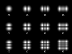
Hermite–Gaussian modes are typically designated "TEMlm"; the fundamental Gaussian beam may thus be referred to as TEM00 (where TEM is transverse electro-magnetic). Multiplying ul(x, z) and um(y, z) to get the 2-D mode profile, and removing the normalization so that the leading factor is just called E0, we can write the (l, m) mode in the more accessible form:
In this form, the parameter w0, as before, determines the family of modes, in particular scaling the spatial extent of the fundamental mode's waist and all other mode patterns at z = 0. Given that w0, w(z) and R(z) have the same definitions as for the fundamental Gaussian beam described above. It can be seen that with l = m = 0 we obtain the fundamental Gaussian beam described earlier (since H0 = 1). The only specific difference in the x and y profiles at any z are due to the Hermite polynomial factors for the order numbers l and m. However, there is a change in the evolution of the modes' Gouy phase over z:
where the combined order of the mode N is defined as N = l + m. While the Gouy phase shift for the fundamental (0,0) Gaussian mode only changes by ±π/2 radians over all of z (and only by ±π/4 radians between ±zR), this is increased by the factor N + 1 for the higher order modes.[10]
Hermite Gaussian modes, with their rectangular symmetry, are especially suited for the modal analysis of radiation from lasers whose cavity design is asymmetric in a rectangular fashion. On the other hand, lasers and systems with circular symmetry can better be handled using the set of Laguerre–Gaussian modes introduced in the next section.
Laguerre–Gaussian modes
Intensity profiles of the first 12 Laguerre–Gaussian modes
Beam profiles which are circularly symmetric (or lasers with cavities that are cylindrically symmetric) are often best solved using the Laguerre–Gaussian modal decomposition.[6] These functions are written in cylindrical coordinates using generalized Laguerre polynomials. Each transverse mode is again labelled using two integers, in this case the radial index p ≥ 0 and the azimuthal index l which can be positive or negative (or zero):[20][21]
A Laguerre–Gaussian beam with l=1 and p=0. Red and blue indicate intensity of the electric field with positive and negative phase.
w(z) and R(z) have the same definitions as above. As with the higher-order Hermite–Gaussian modes the magnitude of the Laguerre–Gaussian modes' Gouy phase shift is exaggerated by the factor N + 1: where in this case the combined mode number N = |l| + 2p. As before, the transverse amplitude variations are contained in the last two factors on the upper line of the equation, which again includes the basic Gaussian drop off in r but now multiplied by a Laguerre polynomial. The effect of the rotational mode number l, in addition to affecting the Laguerre polynomial, is mainly contained in the phase factor exp(−ilφ), in which the beam profile is advanced (or retarded) by l complete 2π phases in one rotation around the beam (in φ). This is an example of an optical vortex of topological charge l, and can be associated with the orbital angular momentum of light in that mode.
Ince–Gaussian modes
Transverse amplitude profile of the lowest order even Ince–Gaussian modes
The third complete family of solution for the paraxial wave equation is the Ince–Gaussian modes. They describe beams with elliptic transverse geometry caracterized by the ellipticity . The Hermite–Gaussian and Laguerre–Gaussian modes are a special case of the Ince–Gaussian modes for and respectively. The Ince–Gaussian modes can be written using elliptic coordinates and Ince polynomials. The even and odd Ince–Gaussian modes and are given by:[7]
where , are normalization constants and , the even and odd Ince polynomials of order and respectively. is the Gouy phase and , are the radial and angular elliptic coordinates defined by:
These modes have a singular phase profile and are eigenfunctions of the photon orbital angular momentum. Their intensity profiles are characterized by a single brilliant ring; like Laguerre–Gaussian modes, their intensities fall to zero at the center (on the optical axis) except for the fundamental (0,0) mode. A mode's complex amplitude can be written in terms of the normalized (dimensionless) radial coordinate and the normalized longitudinal coordinate as follows:[23]
where the rotational index m is an integer, and is real-valued, Γ(x) is the gamma function and 1F1(a, b; x) is a confluent hypergeometric function.
Some subfamilies of hypergeometric-Gaussian (HyGG) modes can be listed as the modified Bessel–Gaussian modes, the modified exponential Gaussian modes,[23] and the modified Laguerre–Gaussian modes.
The set of hypergeometric-Gaussian modes is overcomplete and is not an orthogonal set of modes. In spite of its complicated field profile, HyGG modes have a very simple profile at the beam waist (z = 0):
↑Yariv, Amnon; Yeh, Albert Pochi (2003). Optical Waves in Crystals: Propagation and Control of Laser Radiation. J. Wiley & Sons. ISBN0-471-43081-1. OCLC492184223.
↑Note that the normalization used here (total intensity for a fixed z equal to unity) differs from that used in section #Mathematical form for the Gaussian mode. For l = p = 0 the Laguerre–Gaussian mode reduces to the standard Gaussian mode, but due to different normalization conditions the two formulas do not coincide.
Saleh, Bahaa E. A.; Teich, Malvin Carl (1991). Fundamentals of Photonics. New York: John Wiley & Sons. ISBN0-471-83965-5. Chapter 3, "Beam Optics," pp.80–107.
Siegman, Anthony E. (1986). Lasers. University Science Books. ISBN0-935702-11-3. Chapter 16.
Svelto, Orazio (2010). Principles of Lasers (5thed.).
This page is based on this Wikipedia article Text is available under the CC BY-SA 4.0 license; additional terms may apply. Images, videos and audio are available under their respective licenses.