In probability theory, the expected value of a random variable , denoted or , is a generalization of the weighted average, and is intuitively the arithmetic mean of a large number of independent realizations of . The expected value is also known as the expectation, mathematical expectation, mean, average, or first moment. Expected value is a key concept in economics, finance, and many other subjects.

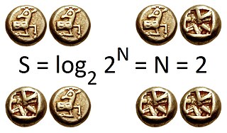
In information theory, the entropy of a random variable is the average level of "information", "surprise", or "uncertainty" inherent in the variable's possible outcomes. The concept of information entropy was introduced by Claude Shannon in his 1948 paper "A Mathematical Theory of Communication". As an example, consider a biased coin with probability p of landing on heads and probability 1-p of landing on tails. The maximum surprise is for p = 1/2, when there is no reason to expect one outcome over another, and in this case a coin flip has an entropy of one bit. The minimum surprise is when p = 0 or p = 1, when the event is known and the entropy is zero bits. Other values of p give different entropies between zero and one bits.

In probability and statistics, a random variable, random quantity, aleatory variable, or stochastic variable is described informally as a variable whose values depend on outcomes of a random phenomenon. The formal mathematical treatment of random variables is a topic in probability theory. In that context, a random variable is understood as a measurable function defined on a probability space that maps from the sample space to the real numbers.
Independence is a fundamental notion in probability theory, as in statistics and the theory of stochastic processes.
In probability theory, the central limit theorem (CLT) establishes that, in many situations, when independent random variables are added, their properly normalized sum tends toward a normal distribution even if the original variables themselves are not normally distributed. The theorem is a key concept in probability theory because it implies that probabilistic and statistical methods that work for normal distributions can be applicable to many problems involving other types of distributions.

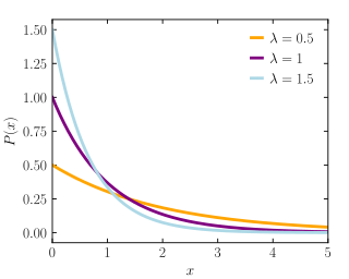
In probability theory and statistics, the exponential distribution is the probability distribution of the time between events in a Poisson point process, i.e., a process in which events occur continuously and independently at a constant average rate. It is a particular case of the gamma distribution. It is the continuous analogue of the geometric distribution, and it has the key property of being memoryless. In addition to being used for the analysis of Poisson point processes it is found in various other contexts.

In probability theory and statistics, the geometric distribution is either one of two discrete probability distributions:

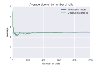
In probability theory, the law of large numbers (LLN) is a theorem that describes the result of performing the same experiment a large number of times. According to the law, the average of the results obtained from a large number of trials should be close to the expected value and will tend to become closer to the expected value as more trials are performed.

In probability theory and statistics, the beta distribution is a family of continuous probability distributions defined on the interval [0, 1] parameterized by two positive shape parameters, denoted by α and β, that appear as exponents of the random variable and control the shape of the distribution. The generalization to multiple variables is called a Dirichlet distribution.
In probability theory, the probability generating function of a discrete random variable is a power series representation of the probability mass function of the random variable. Probability generating functions are often employed for their succinct description of the sequence of probabilities Pr(X = i) in the probability mass function for a random variable X, and to make available the well-developed theory of power series with non-negative coefficients.
In probability theory and statistics, the cumulantsκn of a probability distribution are a set of quantities that provide an alternative to the moments of the distribution. The moments determine the cumulants in the sense that any two probability distributions whose moments are identical will have identical cumulants as well, and similarly the cumulants determine the moments.
In probability theory and statistics, given two jointly distributed random variables and , the conditional probability distribution of Y given X is the probability distribution of when is known to be a particular value; in some cases the conditional probabilities may be expressed as functions containing the unspecified value of as a parameter. When both and are categorical variables, a conditional probability table is typically used to represent the conditional probability. The conditional distribution contrasts with the marginal distribution of a random variable, which is its distribution without reference to the value of the other variable.
In probability theory and statistics, the marginal distribution of a subset of a collection of random variables is the probability distribution of the variables contained in the subset. It gives the probabilities of various values of the variables in the subset without reference to the values of the other variables. This contrasts with a conditional distribution, which gives the probabilities contingent upon the values of the other variables.
In information theory, the information content, self-information, surprisal, or Shannon information is a basic quantity derived from the probability of a particular event occurring from a random variable. It can be thought of as an alternative way of expressing probability, much like odds or log-odds, but which has particular mathematical advantages in the setting of information theory.
In probability theory, a compound Poisson distribution is the probability distribution of the sum of a number of independent identically-distributed random variables, where the number of terms to be added is itself a Poisson-distributed variable. In the simplest cases, the result can be either a continuous or a discrete distribution.
In probability theory, the multinomial distribution is a generalization of the binomial distribution. For example, it models the probability of counts for each side of a k-sided die rolled n times. For n independent trials each of which leads to a success for exactly one of k categories, with each category having a given fixed success probability, the multinomial distribution gives the probability of any particular combination of numbers of successes for the various categories.
In mathematical statistics, the Kullback–Leibler divergence,, is a measure of how one probability distribution is different from a second, reference probability distribution. Applications include characterizing the relative (Shannon) entropy in information systems, randomness in continuous time-series, and information gain when comparing statistical models of inference. In contrast to variation of information, it is a distribution-wise asymmetric measure and thus does not qualify as a statistical metric of spread – it also does not satisfy the triangle inequality. In the simple case, a relative entropy of 0 indicates that the two distributions in question are identical. In simplified terms, it is a measure of surprise, with diverse applications such as applied statistics, fluid mechanics, neuroscience and machine learning.

In probability theory and statistics, the Poisson distribution, named after French mathematician Siméon Denis Poisson, is a discrete probability distribution that expresses the probability of a given number of events occurring in a fixed interval of time or space if these events occur with a known constant mean rate and independently of the time since the last event. The Poisson distribution can also be used for the number of events in other specified intervals such as distance, area or volume.
In probability theory, conditional probability is a measure of the probability of an event occurring, given that another event has already occurred. If the event of interest is A and the event B is known or assumed to have occurred, "the conditional probability of A given B", or "the probability of A under the condition B", is usually written as P(A|B), or sometimes PB(A) or P(A/B). For example, the probability that any given person has a cough on any given day may be only 5%. But if we know or assume that the person is sick, then they are much more likely to be coughing. For example, the conditional probability that someone unwell is coughing might be 75%, in which case we would have that P(Cough) = 5% and P(Cough|Sick) = 75%.
A product distribution is a probability distribution constructed as the distribution of the product of random variables having two other known distributions. Given two statistically independent random variables X and Y, the distribution of the random variable Z that is formed as the product


