In mathematics, the determinant is a scalar-valued function of the entries of a square matrix. The determinant of a matrix A is commonly denoted det(A), det A, or |A|. Its value characterizes some properties of the matrix and the linear map represented, on a given basis, by the matrix. In particular, the determinant is nonzero if and only if the matrix is invertible and the corresponding linear map is an isomorphism.

In mathematics, the discrete Fourier transform (DFT) converts a finite sequence of equally-spaced samples of a function into a same-length sequence of equally-spaced samples of the discrete-time Fourier transform (DTFT), which is a complex-valued function of frequency. The interval at which the DTFT is sampled is the reciprocal of the duration of the input sequence. An inverse DFT (IDFT) is a Fourier series, using the DTFT samples as coefficients of complex sinusoids at the corresponding DTFT frequencies. It has the same sample-values as the original input sequence. The DFT is therefore said to be a frequency domain representation of the original input sequence. If the original sequence spans all the non-zero values of a function, its DTFT is continuous, and the DFT provides discrete samples of one cycle. If the original sequence is one cycle of a periodic function, the DFT provides all the non-zero values of one DTFT cycle.
In mathematics, and more specifically in linear algebra, a linear map is a mapping between two vector spaces that preserves the operations of vector addition and scalar multiplication. The same names and the same definition are also used for the more general case of modules over a ring; see Module homomorphism.

In mathematical physics and mathematics, the Pauli matrices are a set of three 2 × 2 complex matrices that are traceless, Hermitian, involutory and unitary. Usually indicated by the Greek letter sigma, they are occasionally denoted by tau when used in connection with isospin symmetries.

In probability theory and statistics, the multivariate normal distribution, multivariate Gaussian distribution, or joint normal distribution is a generalization of the one-dimensional (univariate) normal distribution to higher dimensions. One definition is that a random vector is said to be k-variate normally distributed if every linear combination of its k components has a univariate normal distribution. Its importance derives mainly from the multivariate central limit theorem. The multivariate normal distribution is often used to describe, at least approximately, any set of (possibly) correlated real-valued random variables, each of which clusters around a mean value.

In geometry, a normal is an object that is perpendicular to a given object. For example, the normal line to a plane curve at a given point is the line perpendicular to the tangent line to the curve at the point.
In mathematics, the name symplectic group can refer to two different, but closely related, collections of mathematical groups, denoted Sp(2n, F) and Sp(n) for positive integer n and field F (usually C or R). The latter is called the compact symplectic group and is also denoted by . Many authors prefer slightly different notations, usually differing by factors of 2. The notation used here is consistent with the size of the most common matrices which represent the groups. In Cartan's classification of the simple Lie algebras, the Lie algebra of the complex group Sp(2n, C) is denoted Cn, and Sp(n) is the compact real form of Sp(2n, C). Note that when we refer to the (compact) symplectic group it is implied that we are talking about the collection of (compact) symplectic groups, indexed by their dimension n.
In mathematics, particularly linear algebra, an orthonormal basis for an inner product space with finite dimension is a basis for whose vectors are orthonormal, that is, they are all unit vectors and orthogonal to each other. For example, the standard basis for a Euclidean space is an orthonormal basis, where the relevant inner product is the dot product of vectors. The image of the standard basis under a rotation or reflection is also orthonormal, and every orthonormal basis for arises in this fashion. An orthonormal basis can be derived from an orthogonal basis via normalization. The choice of an origin and an orthonormal basis forms a coordinate frame known as an orthonormal frame.
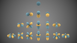
In mathematics and physical science, spherical harmonics are special functions defined on the surface of a sphere. They are often employed in solving partial differential equations in many scientific fields. The table of spherical harmonics contains a list of common spherical harmonics.
In mathematics, the conjugate transpose, also known as the Hermitian transpose, of an complex matrix is an matrix obtained by transposing and applying complex conjugation to each entry. There are several notations, such as or , , or .

The rank–nullity theorem is a theorem in linear algebra, which asserts:
In mathematics, and in particular linear algebra, the Moore–Penrose inverse of a matrix , often called the pseudoinverse, is the most widely known generalization of the inverse matrix. It was independently described by E. H. Moore in 1920, Arne Bjerhammar in 1951, and Roger Penrose in 1955. Earlier, Erik Ivar Fredholm had introduced the concept of a pseudoinverse of integral operators in 1903. The terms pseudoinverse and generalized inverse are sometimes used as synonyms for the Moore–Penrose inverse of a matrix, but sometimes applied to other elements of algebraic structures which share some but not all properties expected for an inverse element.
In mathematics, a homogeneous function is a function of several variables such that the following holds: If each of the function's arguments is multiplied by the same scalar, then the function's value is multiplied by some power of this scalar; the power is called the degree of homogeneity, or simply the degree. That is, if k is an integer, a function f of n variables is homogeneous of degree k if

In geometry, a barycentric coordinate system is a coordinate system in which the location of a point is specified by reference to a simplex. The barycentric coordinates of a point can be interpreted as masses placed at the vertices of the simplex, such that the point is the center of mass of these masses. These masses can be zero or negative; they are all positive if and only if the point is inside the simplex.
In mathematics, the kernel of a linear map, also known as the null space or nullspace, is the part of the domain which is mapped to the zero vector of the co-domain; the kernel is always a linear subspace of the domain. That is, given a linear map L : V → W between two vector spaces V and W, the kernel of L is the vector space of all elements v of V such that L(v) = 0, where 0 denotes the zero vector in W, or more symbolically:
In linear algebra, a generalized eigenvector of an matrix is a vector which satisfies certain criteria which are more relaxed than those for an (ordinary) eigenvector.

In geometry, the hyperboloid model, also known as the Minkowski model after Hermann Minkowski, is a model of n-dimensional hyperbolic geometry in which points are represented by points on the forward sheet S+ of a two-sheeted hyperboloid in (n+1)-dimensional Minkowski space or by the displacement vectors from the origin to those points, and m-planes are represented by the intersections of (m+1)-planes passing through the origin in Minkowski space with S+ or by wedge products of m vectors. Hyperbolic space is embedded isometrically in Minkowski space; that is, the hyperbolic distance function is inherited from Minkowski space, analogous to the way spherical distance is inherited from Euclidean distance when the n-sphere is embedded in (n+1)-dimensional Euclidean space.
In mathematics, a system of equations is considered overdetermined if there are more equations than unknowns. An overdetermined system is almost always inconsistent when constructed with random coefficients. However, an overdetermined system will have solutions in some cases, for example if some equation occurs several times in the system, or if some equations are linear combinations of the others.

In mathematics, an ordinary differential equation (ODE) is a differential equation (DE) dependent on only a single independent variable. As with other DE, its unknown(s) consists of one function(s) and involves the derivatives of those functions. The term "ordinary" is used in contrast with partial differential equations (PDEs) which may be with respect to more than one independent variable, and, less commonly, in contrast with stochastic differential equations (SDEs) where the progression is random.
In linear algebra, a convergent matrix is a matrix that converges to the zero matrix under matrix exponentiation.


