
In physics, the Lorentz transformations are a six-parameter family of linear transformations from a coordinate frame in spacetime to another frame that moves at a constant velocity relative to the former. The respective inverse transformation is then parameterized by the negative of this velocity. The transformations are named after the Dutch physicist Hendrik Lorentz.

In mathematics, the cross product or vector product is a binary operation on two vectors in a three-dimensional oriented Euclidean vector space, and is denoted by the symbol . Given two linearly independent vectors a and b, the cross product, a × b, is a vector that is perpendicular to both a and b, and thus normal to the plane containing them. It has many applications in mathematics, physics, engineering, and computer programming. It should not be confused with the dot product.
In linear algebra, Cramer's rule is an explicit formula for the solution of a system of linear equations with as many equations as unknowns, valid whenever the system has a unique solution. It expresses the solution in terms of the determinants of the (square) coefficient matrix and of matrices obtained from it by replacing one column by the column vector of right-hand-sides of the equations. It is named after Gabriel Cramer (1704–1752), who published the rule for an arbitrary number of unknowns in 1750, although Colin Maclaurin also published special cases of the rule in 1748.
In statistics, the Gauss–Markov theorem states that the ordinary least squares (OLS) estimator has the lowest sampling variance within the class of linear unbiased estimators, if the errors in the linear regression model are uncorrelated, have equal variances and expectation value of zero. The errors do not need to be normal, nor do they need to be independent and identically distributed. The requirement that the estimator be unbiased cannot be dropped, since biased estimators exist with lower variance. See, for example, the James–Stein estimator, ridge regression, or simply any degenerate estimator.

For statistics and control theory, Kalman filtering, also known as linear quadratic estimation (LQE), is an algorithm that uses a series of measurements observed over time, including statistical noise and other inaccuracies, and produces estimates of unknown variables that tend to be more accurate than those based on a single measurement alone, by estimating a joint probability distribution over the variables for each timeframe. The filter is named after Rudolf E. Kálmán, who was one of the primary developers of its theory.
In vector calculus, the Jacobian matrix of a vector-valued function of several variables is the matrix of all its first-order partial derivatives. When this matrix is square, that is, when the function takes the same number of variables as input as the number of vector components of its output, its determinant is referred to as the Jacobian determinant. Both the matrix and the determinant are often referred to simply as the Jacobian in literature.
In the mathematical field of differential geometry, one definition of a metric tensor is a type of function which takes as input a pair of tangent vectors v and w at a point of a surface and produces a real number scalar g(v, w) in a way that generalizes many of the familiar properties of the dot product of vectors in Euclidean space. In the same way as a dot product, metric tensors are used to define the length of tangent vectors and angle between them. Through integration, the metric tensor allows one to define and compute the length of curves on the manifold.
In mathematics, the Heisenberg group, named after Werner Heisenberg, is the group of 3×3 upper triangular matrices of the form

In linear algebra and functional analysis, a projection is a linear transformation from a vector space to itself such that . That is, whenever is applied twice to any vector, it gives the same result as if it were applied once. It leaves its image unchanged. This definition of "projection" formalizes and generalizes the idea of graphical projection. One can also consider the effect of a projection on a geometrical object by examining the effect of the projection on points in the object.
In control engineering, a state-space representation is a mathematical model of a physical system as a set of input, output and state variables related by first-order differential equations or difference equations. State variables are variables whose values evolve over time in a way that depends on the values they have at any given time and on the externally imposed values of input variables. Output variables’ values depend on the values of the state variables.
In mathematics, the matrix exponential is a matrix function on square matrices analogous to the ordinary exponential function. It is used to solve systems of linear differential equations. In the theory of Lie groups, the matrix exponential gives the connection between a matrix Lie algebra and the corresponding Lie group.
In linear algebra, linear transformations can be represented by matrices. If is a linear transformation mapping to and is a column vector with entries, then
In linear algebra, a rotation matrix is a transformation matrix that is used to perform a rotation in Euclidean space. For example, using the convention below, the matrix

In applied statistics, total least squares is a type of errors-in-variables regression, a least squares data modeling technique in which observational errors on both dependent and independent variables are taken into account. It is a generalization of Deming regression and also of orthogonal regression, and can be applied to both linear and non-linear models.
In mathematics, the kernel of a linear map, also known as the null space or nullspace, is the linear subspace of the domain of the map which is mapped to the zero vector. That is, given a linear map L : V → W between two vector spaces V and W, the kernel of L is the vector space of all elements v of V such that L(v) = 0, where 0 denotes the zero vector in W, or more symbolically:
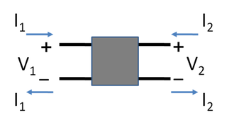
A two-port network is an electrical network (circuit) or device with two pairs of terminals to connect to external circuits. Two terminals constitute a port if the currents applied to them satisfy the essential requirement known as the port condition: the electric current entering one terminal must equal the current emerging from the other terminal on the same port. The ports constitute interfaces where the network connects to other networks, the points where signals are applied or outputs are taken. In a two-port network, often port 1 is considered the input port and port 2 is considered the output port.
In mathematics, matrix calculus is a specialized notation for doing multivariable calculus, especially over spaces of matrices. It collects the various partial derivatives of a single function with respect to many variables, and/or of a multivariate function with respect to a single variable, into vectors and matrices that can be treated as single entities. This greatly simplifies operations such as finding the maximum or minimum of a multivariate function and solving systems of differential equations. The notation used here is commonly used in statistics and engineering, while the tensor index notation is preferred in physics.
As one of the methods of structural analysis, the direct stiffness method, also known as the matrix stiffness method, is particularly suited for computer-automated analysis of complex structures including the statically indeterminate type. It is a matrix method that makes use of the members' stiffness relations for computing member forces and displacements in structures. The direct stiffness method is the most common implementation of the finite element method (FEM). In applying the method, the system must be modeled as a set of simpler, idealized elements interconnected at the nodes. The material stiffness properties of these elements are then, through matrix mathematics, compiled into a single matrix equation which governs the behaviour of the entire idealized structure. The structure’s unknown displacements and forces can then be determined by solving this equation. The direct stiffness method forms the basis for most commercial and free source finite element software.
In geometry, various formalisms exist to express a rotation in three dimensions as a mathematical transformation. In physics, this concept is applied to classical mechanics where rotational kinematics is the science of quantitative description of a purely rotational motion. The orientation of an object at a given instant is described with the same tools, as it is defined as an imaginary rotation from a reference placement in space, rather than an actually observed rotation from a previous placement in space.
A matrix difference equation is a difference equation in which the value of a vector of variables at one point in time is related to its own value at one or more previous points in time, using matrices. The order of the equation is the maximum time gap between any two indicated values of the variable vector. For example,


