Algorithm
First, assume that the domain has been discretized into a mesh. We will refer to mesh points as nodes. Each node  has a corresponding value
  .
.
The algorithm works just like Dijkstra's algorithm but differs in how the nodes' values are calculated. In Dijkstra's algorithm, a node's value is calculated using a single one of the neighboring nodes. However, in solving the PDE in  , between
  and
and  of the neighboring nodes are used.
Nodes are labeled as far (not yet visited), considered (visited and value tentatively assigned), and accepted (visited and value permanently assigned).
- Assign every node the value of
 and label them as far; for all nodes
  set
set  and label as accepted.
 - For every far node , use the Eikonal update formula to calculate a new value for
 . If
. If  then set
  and label as considered.
 - Let
 be the considered node with the smallest value
  . Label as accepted.
 - For every neighbor of that is not-accepted, calculate a tentative value .
- If then set . If was labeled as far, update the label to considered.
- If there exists a considered node, return to step 3. Otherwise, terminate.
In computational mathematics, an iterative method is a mathematical procedure that uses an initial value to generate a sequence of improving approximate solutions for a class of problems, in which the i-th approximation is derived from the previous ones.

The wave equation is a second-order linear partial differential equation for the description of waves or standing wave fields such as mechanical waves or electromagnetic waves. It arises in fields like acoustics, electromagnetism, and fluid dynamics.

The Level-set method (LSM) is a conceptual framework for using level sets as a tool for numerical analysis of surfaces and shapes. LSM can perform numerical computations involving curves and surfaces on a fixed Cartesian grid without having to parameterize these objects. LSM makes it easier to perform computations on shapes with sharp corners and shapes that change topology. These characteristics make LSM effective for modeling objects that vary in time, such as an airbag inflating or a drop of oil floating in water.
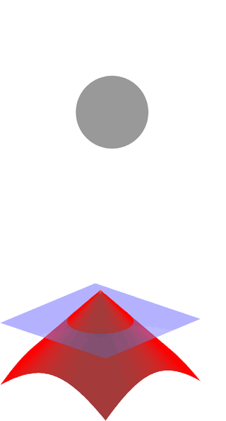
An eikonal equation is a non-linear first-order partial differential equation that is encountered in problems of wave propagation.

The lattice Boltzmann methods (LBM), originated from the lattice gas automata (LGA) method (Hardy-Pomeau-Pazzis and Frisch-Hasslacher-Pomeau models), is a class of computational fluid dynamics (CFD) methods for fluid simulation. Instead of solving the Navier–Stokes equations directly, a fluid density on a lattice is simulated with streaming and collision (relaxation) processes. The method is versatile as the model fluid can straightforwardly be made to mimic common fluid behaviour like vapour/liquid coexistence, and so fluid systems such as liquid droplets can be simulated. Also, fluids in complex environments such as porous media can be straightforwardly simulated, whereas with complex boundaries other CFD methods can be hard to work with.
In mathematics and its applications, the signed distance function or signed distance field (SDF) is the orthogonal distance of a given point x to the boundary of a set Ω in a metric space, with the sign determined by whether or not x is in the interior of Ω. The function has positive values at points x inside Ω, it decreases in value as x approaches the boundary of Ω where the signed distance function is zero, and it takes negative values outside of Ω. However, the alternative convention is also sometimes taken instead. The concept also sometimes goes by the name oriented distance function/field.

The Navier–Stokes existence and smoothness problem concerns the mathematical properties of solutions to the Navier–Stokes equations, a system of partial differential equations that describe the motion of a fluid in space. Solutions to the Navier–Stokes equations are used in many practical applications. However, theoretical understanding of the solutions to these equations is incomplete. In particular, solutions of the Navier–Stokes equations often include turbulence, which remains one of the greatest unsolved problems in physics, despite its immense importance in science and engineering.
In physics, the Spalart–Allmaras model is a one-equation model that solves a modelled transport equation for the kinematic eddy turbulent viscosity. The Spalart–Allmaras model was designed specifically for aerospace applications involving wall-bounded flows and has been shown to give good results for boundary layers subjected to adverse pressure gradients. It is also gaining popularity in turbomachinery applications.
Modified Richardson iteration is an iterative method for solving a system of linear equations. Richardson iteration was proposed by Lewis Fry Richardson in his work dated 1910. It is similar to the Jacobi and Gauss–Seidel method.

In mathematics, an elliptic boundary value problem is a special kind of boundary value problem which can be thought of as the steady state of an evolution problem. For example, the Dirichlet problem for the Laplacian gives the eventual distribution of heat in a room several hours after the heating is turned on.
The topological derivative is, conceptually, a derivative of a shape functional with respect to infinitesimal changes in its topology, such as adding an infinitesimal hole or crack. When used in higher dimensions than one, the term topological gradient is also used to name the first-order term of the topological asymptotic expansion, dealing only with infinitesimal singular domain perturbations. It has applications in shape optimization, topology optimization, image processing and mechanical modeling.
In applied mathematics, discontinuous Galerkin methods (DG methods) form a class of numerical methods for solving differential equations. They combine features of the finite element and the finite volume framework and have been successfully applied to hyperbolic, elliptic, parabolic and mixed form problems arising from a wide range of applications. DG methods have in particular received considerable interest for problems with a dominant first-order part, e.g. in electrodynamics, fluid mechanics and plasma physics. Indeed, the solutions of such problems may involve strong gradients (and even discontinuities) so that classical finite element methods fail, while finite volume methods are restricted to low order approximations.
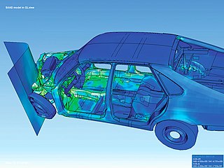
The finite element method (FEM) is a popular method for numerically solving differential equations arising in engineering and mathematical modeling. Typical problem areas of interest include the traditional fields of structural analysis, heat transfer, fluid flow, mass transport, and electromagnetic potential. Computers are usually used to perform the calculations required. With high-speed supercomputers, better solutions can be achieved, and are often required to solve the largest and most complex problems.
In the finite element method for the numerical solution of elliptic partial differential equations, the stiffness matrix is a matrix that represents the system of linear equations that must be solved in order to ascertain an approximate solution to the differential equation.
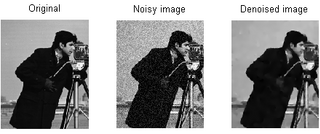
In signal processing, particularly image processing, total variation denoising, also known as total variation regularization or total variation filtering, is a noise removal process (filter). It is based on the principle that signals with excessive and possibly spurious detail have high total variation, that is, the integral of the image gradient magnitude is high. According to this principle, reducing the total variation of the signal—subject to it being a close match to the original signal—removes unwanted detail whilst preserving important details such as edges. The concept was pioneered by L. I. Rudin, S. Osher, and E. Fatemi in 1992 and so is today known as the ROF model.
In numerical mathematics, the boundary knot method (BKM) is proposed as an alternative boundary-type meshfree distance function collocation scheme.
In applied mathematics, the fast sweeping method is a numerical method for solving boundary value problems of the Eikonal equation.

In numerical mathematics, the gradient discretisation method (GDM) is a framework which contains classical and recent numerical schemes for diffusion problems of various kinds: linear or non-linear, steady-state or time-dependent. The schemes may be conforming or non-conforming, and may rely on very general polygonal or polyhedral meshes.
The variational multiscale method (VMS) is a technique used for deriving models and numerical methods for multiscale phenomena. The VMS framework has been mainly applied to design stabilized finite element methods in which stability of the standard Galerkin method is not ensured both in terms of singular perturbation and of compatibility conditions with the finite element spaces.
The Bueno-Orovio–Cherry–Fenton model, also simply called Bueno-Orovio model, is a minimal ionic model for human ventricular cells. It belongs to the category of phenomenological models, because of its characteristic of describing the electrophysiological behaviour of cardiac muscle cells without taking into account in a detailed way the underlying physiology and the specific mechanisms occurring inside the cells.


 Maze as speed function shortest path
 Distance map multi-stencils with random source points
