
In physics, physical chemistry and engineering, fluid dynamics is a subdiscipline of fluid mechanics that describes the flow of fluids — liquids and gases. It has several subdisciplines, including aerodynamics and hydrodynamics. Fluid dynamics has a wide range of applications, including calculating forces and moments on aircraft, determining the mass flow rate of petroleum through pipelines, predicting weather patterns, understanding nebulae in interstellar space and modelling fission weapon detonation.

The Navier–Stokes equations are partial differential equations which describe the motion of viscous fluid substances. They were named after French engineer and physicist Claude-Louis Navier and the Irish physicist and mathematician George Gabriel Stokes. They were developed over several decades of progressively building the theories, from 1822 (Navier) to 1842–1850 (Stokes).
In fluid mechanics, the Grashof number is a dimensionless number which approximates the ratio of the buoyancy to viscous forces acting on a fluid. It frequently arises in the study of situations involving natural convection and is analogous to the Reynolds number.

In fluid dynamics, turbulence or turbulent flow is fluid motion characterized by chaotic changes in pressure and flow velocity. It is in contrast to laminar flow, which occurs when a fluid flows in parallel layers with no disruption between those layers.
The vorticity equation of fluid dynamics describes the evolution of the vorticity ω of a particle of a fluid as it moves with its flow; that is, the local rotation of the fluid. The governing equation is:

In physics and fluid mechanics, a boundary layer is the thin layer of fluid in the immediate vicinity of a bounding surface formed by the fluid flowing along the surface. The fluid's interaction with the wall induces a no-slip boundary condition. The flow velocity then monotonically increases above the surface until it returns to the bulk flow velocity. The thin layer consisting of fluid whose velocity has not yet returned to the bulk flow velocity is called the velocity boundary layer.
The Richardson number (Ri) is named after Lewis Fry Richardson (1881–1953). It is the dimensionless number that expresses the ratio of the buoyancy term to the flow shear term:

In fluid dynamics, the Euler equations are a set of partial differential equations governing adiabatic and inviscid flow. They are named after Leonhard Euler. In particular, they correspond to the Navier–Stokes equations with zero viscosity and zero thermal conductivity.
In fluid mechanics, or more generally continuum mechanics, incompressible flow refers to a flow in which the material density of each fluid parcel — an infinitesimal volume that moves with the flow velocity — is time-invariant. An equivalent statement that implies incompressible flow is that the divergence of the flow velocity is zero.
The Reynolds-averaged Navier–Stokes equations are time-averaged equations of motion for fluid flow. The idea behind the equations is Reynolds decomposition, whereby an instantaneous quantity is decomposed into its time-averaged and fluctuating quantities, an idea first proposed by Osborne Reynolds. The RANS equations are primarily used to describe turbulent flows. These equations can be used with approximations based on knowledge of the properties of flow turbulence to give approximate time-averaged solutions to the Navier–Stokes equations. For a stationary flow of an incompressible Newtonian fluid, these equations can be written in Einstein notation in Cartesian coordinates as:

Large eddy simulation (LES) is a mathematical model for turbulence used in computational fluid dynamics. It was initially proposed in 1963 by Joseph Smagorinsky to simulate atmospheric air currents, and first explored by Deardorff (1970). LES is currently applied in a wide variety of engineering applications, including combustion, acoustics, and simulations of the atmospheric boundary layer.
The Rayleigh–Taylor instability, or RT instability, is an instability of an interface between two fluids of different densities which occurs when the lighter fluid is pushing the heavier fluid. Examples include the behavior of water suspended above oil in the gravity of Earth, mushroom clouds like those from volcanic eruptions and atmospheric nuclear explosions, supernova explosions in which expanding core gas is accelerated into denser shell gas, instabilities in plasma fusion reactors and inertial confinement fusion.
In fluid dynamics, the Reynolds stress is the component of the total stress tensor in a fluid obtained from the averaging operation over the Navier–Stokes equations to account for turbulent fluctuations in fluid momentum.
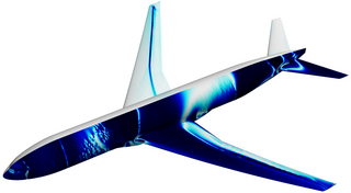
In fluid dynamics, turbulence modeling is the construction and use of a mathematical model to predict the effects of turbulence. Turbulent flows are commonplace in most real-life scenarios. In spite of decades of research, there is no analytical theory to predict the evolution of these turbulent flows. The equations governing turbulent flows can only be solved directly for simple cases of flow. For most real-life turbulent flows, CFD simulations use turbulent models to predict the evolution of turbulence. These turbulence models are simplified constitutive equations that predict the statistical evolution of turbulent flows.
In fluid dynamics, turbulence kinetic energy (TKE) is the mean kinetic energy per unit mass associated with eddies in turbulent flow. Physically, the turbulence kinetic energy is characterized by measured root-mean-square (RMS) velocity fluctuations. In the Reynolds-averaged Navier Stokes equations, the turbulence kinetic energy can be calculated based on the closure method, i.e. a turbulence model.
The turbulent Prandtl number (Prt) is a non-dimensional term defined as the ratio between the momentum eddy diffusivity and the heat transfer eddy diffusivity. It is useful for solving the heat transfer problem of turbulent boundary layer flows. The simplest model for Prt is the Reynolds analogy, which yields a turbulent Prandtl number of 1. From experimental data, Prt has an average value of 0.85, but ranges from 0.7 to 0.9 depending on the Prandtl number of the fluid in question.
Shear velocity, also called friction velocity, is a form by which a shear stress may be re-written in units of velocity. It is useful as a method in fluid mechanics to compare true velocities, such as the velocity of a flow in a stream, to a velocity that relates shear between layers of flow.

In fluid dynamics, hydrodynamic stability is the field which analyses the stability and the onset of instability of fluid flows. The study of hydrodynamic stability aims to find out if a given flow is stable or unstable, and if so, how these instabilities will cause the development of turbulence. The foundations of hydrodynamic stability, both theoretical and experimental, were laid most notably by Helmholtz, Kelvin, Rayleigh and Reynolds during the nineteenth century. These foundations have given many useful tools to study hydrodynamic stability. These include Reynolds number, the Euler equations, and the Navier–Stokes equations. When studying flow stability it is useful to understand more simplistic systems, e.g. incompressible and inviscid fluids which can then be developed further onto more complex flows. Since the 1980s, more computational methods are being used to model and analyse the more complex flows.

In fluid dynamics, the Reynolds number is a dimensionless quantity that helps predict fluid flow patterns in different situations by measuring the ratio between inertial and viscous forces. At low Reynolds numbers, flows tend to be dominated by laminar (sheet-like) flow, while at high Reynolds numbers, flows tend to be turbulent. The turbulence results from differences in the fluid's speed and direction, which may sometimes intersect or even move counter to the overall direction of the flow. These eddy currents begin to churn the flow, using up energy in the process, which for liquids increases the chances of cavitation.

In fluid dynamics, the radiation stress is the depth-integrated – and thereafter phase-averaged – excess momentum flux caused by the presence of the surface gravity waves, which is exerted on the mean flow. The radiation stresses behave as a second-order tensor.


