
In mathematics and physics, Laplace's equation is a second-order partial differential equation named after Pierre-Simon Laplace, who first studied its properties. This is often written as

In mathematics, the Dirac delta distribution, also known as the unit impulse, is a generalized function or distribution over the real numbers, whose value is zero everywhere except at zero, and whose integral over the entire real line is equal to one.

Noether's theorem or Noether's first theorem states that every differentiable symmetry of the action of a physical system with conservative forces has a corresponding conservation law. The theorem was proven by mathematician Emmy Noether in 1915 and published in 1918. The action of a physical system is the integral over time of a Lagrangian function, from which the system's behavior can be determined by the principle of least action. This theorem only applies to continuous and smooth symmetries over physical space.
In mathematics, the Laplace operator or Laplacian is a differential operator given by the divergence of the gradient of a scalar function on Euclidean space. It is usually denoted by the symbols , , or . In a Cartesian coordinate system, the Laplacian is given by the sum of second partial derivatives of the function with respect to each independent variable. In other coordinate systems, such as cylindrical and spherical coordinates, the Laplacian also has a useful form. Informally, the Laplacian Δf (p) of a function f at a point p measures by how much the average value of f over small spheres or balls centered at p deviates from f (p).
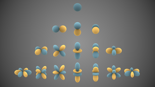
In mathematics and physical science, spherical harmonics are special functions defined on the surface of a sphere. They are often employed in solving partial differential equations in many scientific fields.
Linear elasticity is a mathematical model of how solid objects deform and become internally stressed due to prescribed loading conditions. It is a simplification of the more general nonlinear theory of elasticity and a branch of continuum mechanics.
In the calculus of variations, a field of mathematical analysis, the functional derivative relates a change in a functional to a change in a function on which the functional depends.

In mathematics, a Green's function is the impulse response of an inhomogeneous linear differential operator defined on a domain with specified initial conditions or boundary conditions.

The path integral formulation is a description in quantum mechanics that generalizes the action principle of classical mechanics. It replaces the classical notion of a single, unique classical trajectory for a system with a sum, or functional integral, over an infinity of quantum-mechanically possible trajectories to compute a quantum amplitude.
In the statistical analysis of time series, autoregressive–moving-average (ARMA) models provide a parsimonious description of a (weakly) stationary stochastic process in terms of two polynomials, one for the autoregression (AR) and the second for the moving average (MA). The general ARMA model was described in the 1951 thesis of Peter Whittle, Hypothesis testing in time series analysis, and it was popularized in the 1970 book by George E. P. Box and Gwilym Jenkins.
In statistics, econometrics and signal processing, an autoregressive (AR) model is a representation of a type of random process; as such, it is used to describe certain time-varying processes in nature, economics, etc. The autoregressive model specifies that the output variable depends linearly on its own previous values and on a stochastic term ; thus the model is in the form of a stochastic difference equation. Together with the moving-average (MA) model, it is a special case and key component of the more general autoregressive–moving-average (ARMA) and autoregressive integrated moving average (ARIMA) models of time series, which have a more complicated stochastic structure; it is also a special case of the vector autoregressive model (VAR), which consists of a system of more than one interlocking stochastic difference equation in more than one evolving random variable.
In statistics and econometrics, and in particular in time series analysis, an autoregressive integrated moving average (ARIMA) model is a generalization of an autoregressive moving average (ARMA) model. Both of these models are fitted to time series data either to better understand the data or to predict future points in the series (forecasting). ARIMA models are applied in some cases where data show evidence of non-stationarity in the sense of mean, where an initial differencing step can be applied one or more times to eliminate the non-stationarity of the mean function. When the seasonality shows in a time series, the seasonal-differencing could be applied to eliminate the seasonal component. Since the ARMA model, according to the Wold's decomposition theorem, is theoretically sufficient to describe a regular wide-sense stationary time series, we are motivated to make stationary a non-stationary time series, e.g., by using differencing, before we can use the ARMA model. Note that if the time series contains a predictable sub-process, the predictable component is treated as a non-zero-mean but periodic component in the ARIMA framework so that it is eliminated by the seasonal differencing.

Arc length is the distance between two points along a section of a curve.
Uncertainty quantification (UQ) is the science of quantitative characterization and reduction of uncertainties in both computational and real world applications. It tries to determine how likely certain outcomes are if some aspects of the system are not exactly known. An example would be to predict the acceleration of a human body in a head-on crash with another car: even if the speed was exactly known, small differences in the manufacturing of individual cars, how tightly every bolt has been tightened, etc., will lead to different results that can only be predicted in a statistical sense.
In physics, the Green's function for Laplace's equation in three variables is used to describe the response of a particular type of physical system to a point source. In particular, this Green's function arises in systems that can be described by Poisson's equation, a partial differential equation (PDE) of the form
In mathematics, vector spherical harmonics (VSH) are an extension of the scalar spherical harmonics for use with vector fields. The components of the VSH are complex-valued functions expressed in the spherical coordinate basis vectors.
In time series analysis, the moving-average model, also known as moving-average process, is a common approach for modeling univariate time series. The moving-average model specifies that the output variable is cross-correlated with a non-identical to itself random-variable.
In mathematics, the Butcher group, named after the New Zealand mathematician John C. Butcher by Hairer & Wanner (1974), is an infinite-dimensional Lie group first introduced in numerical analysis to study solutions of non-linear ordinary differential equations by the Runge–Kutta method. It arose from an algebraic formalism involving rooted trees that provides formal power series solutions of the differential equation modeling the flow of a vector field. It was Cayley (1857), prompted by the work of Sylvester on change of variables in differential calculus, who first noted that the derivatives of a composition of functions can be conveniently expressed in terms of rooted trees and their combinatorics.
In mathematics, singular integral operators of convolution type are the singular integral operators that arise on Rn and Tn through convolution by distributions; equivalently they are the singular integral operators that commute with translations. The classical examples in harmonic analysis are the harmonic conjugation operator on the circle, the Hilbert transform on the circle and the real line, the Beurling transform in the complex plane and the Riesz transforms in Euclidean space. The continuity of these operators on L2 is evident because the Fourier transform converts them into multiplication operators. Continuity on Lp spaces was first established by Marcel Riesz. The classical techniques include the use of Poisson integrals, interpolation theory and the Hardy–Littlewood maximal function. For more general operators, fundamental new techniques, introduced by Alberto Calderón and Antoni Zygmund in 1952, were developed by a number of authors to give general criteria for continuity on Lp spaces. This article explains the theory for the classical operators and sketches the subsequent general theory.
In mathematics, singular integral operators on closed curves arise in problems in analysis, in particular complex analysis and harmonic analysis. The two main singular integral operators, the Hilbert transform and the Cauchy transform, can be defined for any smooth Jordan curve in the complex plane and are related by a simple algebraic formula. In the special case of Fourier series for the unit circle, the operators become the classical Cauchy transform, the orthogonal projection onto Hardy space, and the Hilbert transform a real orthogonal linear complex structure. In general the Cauchy transform is a non-self-adjoint idempotent and the Hilbert transform a non-orthogonal complex structure. The range of the Cauchy transform is the Hardy space of the bounded region enclosed by the Jordan curve. The theory for the original curve can be deduced from that of the unit circle, where, because of rotational symmetry, both operators are classical singular integral operators of convolution type. The Hilbert transform satisfies the jump relations of Plemelj and Sokhotski, which express the original function as the difference between the boundary values of holomorphic functions on the region and its complement. Singular integral operators have been studied on various classes of functions, including Hőlder spaces, Lp spaces and Sobolev spaces. In the case of L2 spaces—the case treated in detail below—other operators associated with the closed curve, such as the Szegő projection onto Hardy space and the Neumann–Poincaré operator, can be expressed in terms of the Cauchy transform and its adjoint.


