The method of least squares is a parameters estimation method in regression analysis based on minimizing the sum of the squares of the residuals made in the results of each individual equation.

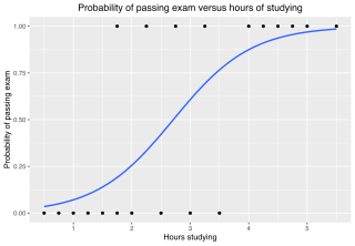
In statistics, the logistic model is a statistical model that models the log-odds of an event as a linear combination of one or more independent variables. In regression analysis, logistic regression is estimating the parameters of a logistic model. Formally, in binary logistic regression there is a single binary dependent variable, coded by an indicator variable, where the two values are labeled "0" and "1", while the independent variables can each be a binary variable or a continuous variable. The corresponding probability of the value labeled "1" can vary between 0 and 1, hence the labeling; the function that converts log-odds to probability is the logistic function, hence the name. The unit of measurement for the log-odds scale is called a logit, from logistic unit, hence the alternative names. See § Background and § Definition for formal mathematics, and § Example for a worked example.

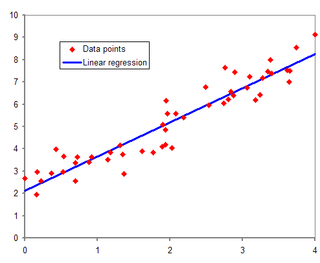
In statistical modeling, regression analysis is a set of statistical processes for estimating the relationships between a dependent variable and one or more independent variables. The most common form of regression analysis is linear regression, in which one finds the line that most closely fits the data according to a specific mathematical criterion. For example, the method of ordinary least squares computes the unique line that minimizes the sum of squared differences between the true data and that line. For specific mathematical reasons, this allows the researcher to estimate the conditional expectation of the dependent variable when the independent variables take on a given set of values. Less common forms of regression use slightly different procedures to estimate alternative location parameters or estimate the conditional expectation across a broader collection of non-linear models.
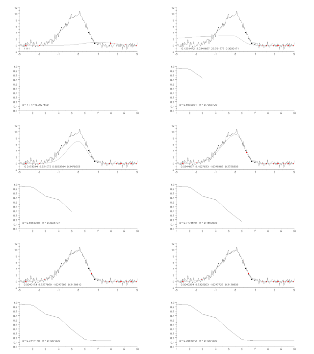
In mathematics and computing, the Levenberg–Marquardt algorithm, also known as the damped least-squares (DLS) method, is used to solve non-linear least squares problems. These minimization problems arise especially in least squares curve fitting. The LMA interpolates between the Gauss–Newton algorithm (GNA) and the method of gradient descent. The LMA is more robust than the GNA, which means that in many cases it finds a solution even if it starts very far off the final minimum. For well-behaved functions and reasonable starting parameters, the LMA tends to be slower than the GNA. LMA can also be viewed as Gauss–Newton using a trust region approach.

In applied statistics, total least squares is a type of errors-in-variables regression, a least squares data modeling technique in which observational errors on both dependent and independent variables are taken into account. It is a generalization of Deming regression and also of orthogonal regression, and can be applied to both linear and non-linear models.

In statistics, nonlinear regression is a form of regression analysis in which observational data are modeled by a function which is a nonlinear combination of the model parameters and depends on one or more independent variables. The data are fitted by a method of successive approximations.

The Gauss–Newton algorithm is used to solve non-linear least squares problems, which is equivalent to minimizing a sum of squared function values. It is an extension of Newton's method for finding a minimum of a non-linear function. Since a sum of squares must be nonnegative, the algorithm can be viewed as using Newton's method to iteratively approximate zeroes of the components of the sum, and thus minimizing the sum. In this sense, the algorithm is also an effective method for solving overdetermined systems of equations. It has the advantage that second derivatives, which can be challenging to compute, are not required.

In statistics, the coefficient of determination, denoted R2 or r2 and pronounced "R squared", is the proportion of the variation in the dependent variable that is predictable from the independent variable(s).
In statistics, ordinary least squares (OLS) is a type of linear least squares method for choosing the unknown parameters in a linear regression model by the principle of least squares: minimizing the sum of the squares of the differences between the observed dependent variable in the input dataset and the output of the (linear) function of the independent variable.
Weighted least squares (WLS), also known as weighted linear regression, is a generalization of ordinary least squares and linear regression in which knowledge of the unequal variance of observations (heteroscedasticity) is incorporated into the regression. WLS is also a specialization of generalized least squares, when all the off-diagonal entries of the covariance matrix of the errors, are null.

In statistics, simple linear regression (SLR) is a linear regression model with a single explanatory variable. That is, it concerns two-dimensional sample points with one independent variable and one dependent variable and finds a linear function that, as accurately as possible, predicts the dependent variable values as a function of the independent variable. The adjective simple refers to the fact that the outcome variable is related to a single predictor.
In robust statistics, robust regression seeks to overcome some limitations of traditional regression analysis. A regression analysis models the relationship between one or more independent variables and a dependent variable. Standard types of regression, such as ordinary least squares, have favourable properties if their underlying assumptions are true, but can give misleading results otherwise. Robust regression methods are designed to limit the effect that violations of assumptions by the underlying data-generating process have on regression estimates.
Robust statistics are statistics which maintain their properties even if the underlying distributional assumptions are incorrect. Robust statistical methods have been developed for many common problems, such as estimating location, scale, and regression parameters. One motivation is to produce statistical methods that are not unduly affected by outliers. Another motivation is to provide methods with good performance when there are small departures from a parametric distribution. For example, robust methods work well for mixtures of two normal distributions with different standard deviations; under this model, non-robust methods like a t-test work poorly.
The method of iteratively reweighted least squares (IRLS) is used to solve certain optimization problems with objective functions of the form of a p-norm:
The topic of heteroskedasticity-consistent (HC) standard errors arises in statistics and econometrics in the context of linear regression and time series analysis. These are also known as heteroskedasticity-robust standard errors, Eicker–Huber–White standard errors, to recognize the contributions of Friedhelm Eicker, Peter J. Huber, and Halbert White.
Non-linear least squares is the form of least squares analysis used to fit a set of m observations with a model that is non-linear in n unknown parameters (m ≥ n). It is used in some forms of nonlinear regression. The basis of the method is to approximate the model by a linear one and to refine the parameters by successive iterations. There are many similarities to linear least squares, but also some significant differences. In economic theory, the non-linear least squares method is applied in (i) the probit regression, (ii) threshold regression, (iii) smooth regression, (iv) logistic link regression, (v) Box–Cox transformed regressors ().
Least absolute deviations (LAD), also known as least absolute errors (LAE), least absolute residuals (LAR), or least absolute values (LAV), is a statistical optimality criterion and a statistical optimization technique based on minimizing the sum of absolute deviations or the L1 norm of such values. It is analogous to the least squares technique, except that it is based on absolute values instead of squared values. It attempts to find a function which closely approximates a set of data by minimizing residuals between points generated by the function and corresponding data points. The LAD estimate also arises as the maximum likelihood estimate if the errors have a Laplace distribution. It was introduced in 1757 by Roger Joseph Boscovich.
In statistics, projection pursuit regression (PPR) is a statistical model developed by Jerome H. Friedman and Werner Stuetzle that extends additive models. This model adapts the additive models in that it first projects the data matrix of explanatory variables in the optimal direction before applying smoothing functions to these explanatory variables.
Linear least squares (LLS) is the least squares approximation of linear functions to data. It is a set of formulations for solving statistical problems involved in linear regression, including variants for ordinary (unweighted), weighted, and generalized (correlated) residuals. Numerical methods for linear least squares include inverting the matrix of the normal equations and orthogonal decomposition methods.

Peter J. Rousseeuw is a statistician known for his work on robust statistics and cluster analysis. He obtained his PhD in 1981 at the Vrije Universiteit Brussel, following research carried out at the ETH in Zurich, which led to a book on influence functions. Later he was professor at the Delft University of Technology, The Netherlands, at the University of Fribourg, Switzerland, and at the University of Antwerp, Belgium. Next he was a senior researcher at Renaissance Technologies. He then returned to Belgium as professor at KU Leuven, until becoming emeritus in 2022. His former PhD students include Annick Leroy, Hendrik Lopuhaä, Geert Molenberghs, Christophe Croux, Mia Hubert, Stefan Van Aelst, Tim Verdonck and Jakob Raymaekers.


