Leftist tree

In computer science, a leftist tree or leftist heap is a priority queue implemented with a variant of a binary heap. Every node x has an s-value which is the distance to the nearest leaf in subtree rooted at x. ^[1] In contrast to a binary heap, a leftist tree attempts to be very unbalanced. In addition to the heap property, leftist trees are maintained so the right descendant of each node has the lower s-value.

The height-biased leftist tree was invented by Clark Allan Crane. ^[2] The name comes from the fact that the left subtree is usually taller than the right subtree.

A leftist tree is a mergeable heap. When inserting a new node into a tree, a new one-node tree is created and merged into the existing tree. To delete an item, it is replaced by the merge of its left and right sub-trees. Both these operations take O(log n) time. For insertions, this is slower than Fibonacci heaps, which support insertion in O(1) (constant) amortized time, and O(log n) worst-case.

Leftist trees are advantageous because of their ability to merge quickly, compared to binary heaps which take Θ(n). In almost all cases, the merging of skew heaps has better performance. However merging leftist heaps has worst-case O(log n) complexity while merging skew heaps has only amortized O(log n) complexity.

Bias

The usual leftist tree is a height-biased leftist tree. ^[2] However, other biases can exist, such as in the weight-biased leftist tree. ^[3]

S-value

S-values of a leftist tree

The s-value (or rank) of a node is the distance from that node to the nearest empty position in the subtree rooted at that node. Put another way, the s-value of a null child is implicitly zero. Other nodes have an s-value equal to one more the minimum of their children's s-values. Thus, in the example at right, all nodes with at least one missing child have an s-value of 1, while node 4 has an s-value of 2, since its right child (8) has an s-value of 1. (In some descriptions, the s-value of null children is assumed to be −1. ^[4] )

Knowing the shortest path to the nearest missing leaf in the subtree rooted at x is exactly of s(x), every node at depth s(x)−1 or less has exactly 2 children since s(x) would have been less if not. Meaning that the size of the tree rooted at x is at least ${\displaystyle 2^{s(x)}-1}$. Thus, s(x) is at most ${\displaystyle \log {(m+1)}}$, m being the number of nodes of the subtree rooted at x. ^[1]

Operations on a height biased leftist tree

Most operations on a Height Biased Leftist Tree are done using the merge operation. ^[1]

Merging two Min HBLTs

The merge operation takes two Min HBLTs as input and returns a Min HBLT containing all the nodes in the original Min HBLTs put together.

If either of A or B is empty, the merge returns the other one.

In case of Min HBLTs, assume we have two trees rooted at A and B where A.key ${\displaystyle \leq }$ B.key. Otherwise we can swap A and B so that the condition above holds.

The merge is done recursively by merging B with A's right subtree. This might change the S-value of A's right subtree. To maintain the leftist tree property, after each merge is done, we check if the S-value of right subtree became bigger than the S-value of left subtree during the recursive merge calls. If so, we swap the right and left subtrees (If one child is missing, it should be the right one).

Since we assumed that A's root is greater than B's, the heap property is also maintained.

Pseudocode for merging two min height biased leftist trees

MERGE(A, B)     if A = null return B     if B = null return A     if A.key > B.key return MERGE(B, A)     A.right := MERGE (A.right, B) // the result cannot be null since B is non-nullif A.left = null then         SWAP(A.left, A.right)         A.s_value := 1 // since the right subtree is null, the shortest path to a descendant leaf from node A is 1return A     if A.right.s_value > A.left.s_value then         SWAP (A.right, A.left)     A.s_value := A.right.s_value + 1     return A

Java code for merging two min height biased leftist trees

publicNodemerge(Nodex,Nodey){if(x==null)returny;if(y==null)returnx;// if this were a max-heap, then the // next line would be: if (x.element < y.element)if(x.element.compareTo(y.element)>0)// x.element > y.elementreturnmerge(y,x);x.rightChild=merge(x.rightChild,y);if(x.leftChild==null){// left child doesn't exist, so move right child to the left sidex.leftChild=x.rightChild;x.rightChild=null;// x.s was, and remains, 1}else{// left child does exist, so compare s-valuesif(x.leftChild.s<x.rightChild.s){Nodetemp=x.leftChild;x.leftChild=x.rightChild;x.rightChild=temp;}// since we know the right child has the lower s-value, we can just// add one to its s-valuex.s=x.rightChild.s+1;}returnx;}

Haskell code for merging two min height biased leftist trees

dataLHeapa=Leaf|Nodea(LHeapa)(LHeapa)rank::LHeapa->IntegerrankLeaf=0rank(Node__r)=rankr+1merge::Orda=>LHeapa->LHeapa->LHeapamergeLeafh=hmergehLeaf=hmergeh@(Nodealr)h'@(Nodea'__)|a>a'=mergeh'h|rankr'>rankl=Nodear'l|otherwise=Nodealr'wherer'=mergerh'

Example

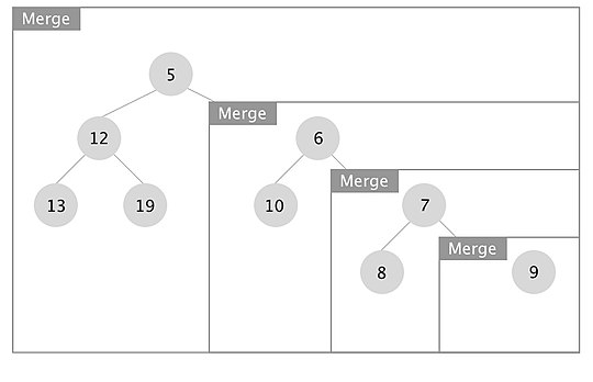
An example of how the merge operation in a leftist tree works is depicted. The boxes represent each merge call.

• 
• 
• 
• 
• 
• 
• 
• 
• 

When the recursion unwinds, we swap left and right children if x.right.s_value > x.left.s_value for every node x. In this case we swapped the subtrees rooted at nodes with keys 7 and 10.

Insertion into a Min HBLT

Insertion is done using the merge operation. An insertion of a node into an already existing

Min HBLT, creates a HBLT tree of size one with that node and merges it with the existing tree.

INSERT (A, x)     B := CREATE_TREE(x)     return MERGE(A, B)

Deletion of Min element from Min HBLT

The Min element in a Min HBLT is the root. Thus, in order to delete the Min, the root is deleted and its subtrees are merged to form the new Min HBLT.

DELETE_MIN(A)     x := A.key     A := MERGE (A.right, A.left)     returnx

Initializing a height biased leftist tree

Initializing a min HBLT - Part 1

Initializing a height biased leftist tree is primarily done in one of two ways. The first is to merge each node one at a time into one HBLT. This process is inefficient and takes O(nlogn) time. The other approach is to use a queue to store each node and resulting tree. The first two items in the queue are removed, merged, and placed back into the queue. This can initialize a HBLT in O(n) time. This approach is detailed in the three diagrams supplied. A min height biased leftist tree is shown.

To initialize a min HBLT, place each element to be added to the tree into a queue. In the example (see Part 1 to the left), the set of numbers [4, 8, 10, 9, 1, 3, 5, 6, 11] are initialized. Each line of the diagram represents another cycle of the algorithm, depicting the contents of the queue. The first five steps are easy to follow. Notice that the freshly created HBLT is added to the end of the queue. In the fifth step, the first occurrence of an s-value greater than 1 occurs. The sixth step shows two trees merged with each other, with predictable results.

Initializing a min HBLT - Part 2

In part 2 a slightly more complex merge happens. The tree with the lower value (tree x) has a right child, so merge must be called again on the subtree rooted by tree x's right child and the other tree. After the merge with the subtree, the resulting tree is put back into tree x. The s-value of the right child (s=2) is now greater than the s-value of the left child (s=1), so they must be swapped. The s-value of the root node 4 is also now 2.

Initializing a min HBLT - Part 3

Part 3 is the most complex. Here, we recursively call merge twice (each time with the right child 's subtree that is not grayed out). This uses the same process described for part 2.

Deletion of an arbitrary element from a Min HBLT

If we have a pointer to a node x in a Min HBLT, we can delete it as follows: Replace the node x with the result of merging its two subtrees and update the s-values of the nodes on the path from x to the root, swapping the right and left subtrees if necessary to maintain the leftist tree property.

The upward traversal is continued until either we hit the root or the s-values does not change. Since we are deleting an element, the S-values on the path traversed cannot be increased. Every node that is already the right child of its parent and causes its parent's s-value to be decreased, will remain on the right. Every node that is its parent's left child and causes the parent's s-value to be decreased has to be swapped with its right sibling if the s-value becomes lower than the current s-value of the right child.

Each node needs to have a pointer to its parent, so that we can traverse the path to the root updating the s-values.

When the traversal ends at some node y, the nodes traversed all lie on the rightmost path rooted at node y. An example is shown below. It follows that the number of nodes traversed is at most log(m), m being the size of the subtree rooted at y. Thus, this operation also takes O(lg m) to perform.

Weight biased leftist tree ^[5]

Leftist trees can also be weight biased. In this case, instead of storing s-values in node x, we store an attribute w(x) denoting the number of nodes in the subtree rooted at x:

w(x) = w(x.right) + w(x.left) + 1

WBLTs ensure w(x.left) ≥ w(x.right) for all internal nodes x. WBLT operations ensure this invariant by swapping the children of a node when the right subtree outgrows the left one, just as in HBLT operations.

Merging two Min WBLTs

The merge operation in WBLTs can be done using a single top to bottom traversal since the number of nodes in the subtrees are known prior to recursive call to merge. Thus, we can swap left and right subtrees if the total number of nodes in the right subtree and the tree to be merged is bigger than the number of nodes in the left subtree. This allows the operations be completed in a single path and so improves the time complexity of the operations by a constant factor.

The merge operation is depicted in the graph below.

• 
• 
• 
• 
• 
• 
• 
• 
• 
• 

Other operations on WBLT

Insertions and deletion of the min element can be done in the same as for HBLTs using the merge operation.

Although WBLTs outperform HBLTs in merge, insertion and deletion of the Min key by a constant factor, the O(log n) bound is not guaranteed when deleting an arbitrary element from WBLTs, since θ(n) nodes have to be traversed.

If this was an HBLT, then deleting the leaf node with key 60 would take O(1) time and updating the s-values is not needed since the length of rightmost path for all the nodes does not change.

But in an WBLT tree, we have to update the weight of each node back to the root, which takes O(n) worst case.

Variants

Several variations on the basic leftist tree exist, which make only minor changes to the basic algorithm:

• The choice of the left child as the taller one is arbitrary; a "rightist tree" would work just as well.
• It is possible to avoid swapping children, but instead record which child is the tallest (in, for example, the least significant bit of the s-value) and use that in the merge operation.
• The s-value used to decide which side to merge with could use a metric other than height. For example, weight (number of nodes) could be used.

References

1. "Leftist Trees" (PDF). www.google.com. Retrieved 2019-05-31.
2. Crane, Clark A. (1972), Linear Lists and Priority Queues as Balanced Binary Trees (Ph.D. thesis), Department of Computer Science, Stanford University, ISBN   0-8240-4407-X, STAN-CS-72-259
3. Seonghun Cho; Sartaj Sahni (1996), "Weight Biased Leftist Trees and Modified Skip Lists" (PDF), Journal of Experimental Algorithmics, 3, CiteSeerX   10.1.1.13.2962 , doi:10.1145/297096.297111
4. Stewart, James (25 September 1988). "LEFTIST TREES". University of Toronto Dynamic Graphics Project. Retrieved 2019-05-31.
5. Cho, Seonghun; Sahni, Sartaj (September 1998). "Weight-biased Leftist Trees and Modified Skip Lists". J. Exp. Algorithmics. 3. doi:10.1145/297096.297111. ISSN   1084-6654.

Further reading

• Robert E. Tarjan (1983). Data Structures and Network Algorithms. SIAM. pp. 38–42. ISBN   978-0-89871-187-5.
• Dinesh P. Mehta; Sartaj Sahni (28 October 2004). "Chapter 5: Leftist trees". Handbook of Data Structures and Applications. CRC Press. ISBN   978-1-4200-3517-9.

External links

• Leftist Trees, Sartaj Sahni