The stimulus–response model is a characterization of a statistical unit. The model allows the prediction of a quantitative response to a quantitative stimulus, for example one administered by a researcher. In psychology, stimulus response theory concerns forms of classical conditioning in which a stimulus becomes paired response in a subject's mind.

Given a collection of points in two, three, or higher dimensional space, a "best fitting" line can be defined as one that minimizes the average squared distance from a point to the line. The next best-fitting line can be similarly chosen from directions perpendicular to the first. Repeating this process yields an orthogonal basis in which different individual dimensions of the data are uncorrelated. These basis vectors are called principal components, and several related procedures principal component analysis (PCA).

In machine learning, the perceptron is an algorithm for supervised learning of binary classifiers. A binary classifier is a function which can decide whether or not an input, represented by a vector of numbers, belongs to some specific class. It is a type of linear classifier, i.e. a classification algorithm that makes its predictions based on a linear predictor function combining a set of weights with the feature vector.
In control engineering, a state-space representation is a mathematical model of a physical system as a set of input, output and state variables related by first-order differential equations or difference equations. State variables are variables whose values evolve through time in a way that depends on the values they have at any given time and also depends on the externally imposed values of input variables. Output variables’ values depend on the values of the state variables.

In statistics, the generalized linear model (GLM) is a flexible generalization of ordinary linear regression that allows for response variables that have error distribution models other than a normal distribution. The GLM generalizes linear regression by allowing the linear model to be related to the response variable via a link function and by allowing the magnitude of the variance of each measurement to be a function of its predicted value.

The Granger causality test is a statistical hypothesis test for determining whether one time series is useful in forecasting another, first proposed in 1969. Ordinarily, regressions reflect "mere" correlations, but Clive Granger argued that causality in economics could be tested for by measuring the ability to predict the future values of a time series using prior values of another time series. Since the question of "true causality" is deeply philosophical, and because of the post hoc ergo propter hoc fallacy of assuming that one thing preceding another can be used as a proof of causation, econometricians assert that the Granger test finds only "predictive causality". Using the term "causality" alone is a misnomer, as Granger-causality is better described as "precedence", or, as Granger himself later claimed in 1977, "temporally related". Rather than testing whether Ycauses X, the Granger causality tests whether Y forecastsX.
A multilayer perceptron (MLP) is a class of feedforward artificial neural network (ANN). The term MLP is used ambiguously, sometimes loosely to any feedforward ANN, sometimes strictly to refer to networks composed of multiple layers of perceptrons ; see § Terminology. Multilayer perceptrons are sometimes colloquially referred to as "vanilla" neural networks, especially when they have a single hidden layer.
In machine learning, kernel methods are a class of algorithms for pattern analysis, whose best known member is the support vector machine (SVM). The general task of pattern analysis is to find and study general types of relations in datasets. For many algorithms that solve these tasks, the data in raw representation have to be explicitly transformed into feature vector representations via a user-specified feature map: in contrast, kernel methods require only a user-specified kernel, i.e., a similarity function over pairs of data points in raw representation.
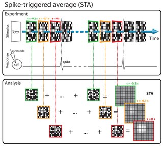
The spike-triggered average (STA) is a tool for characterizing the response properties of a neuron using the spikes emitted in response to a time-varying stimulus. The STA provides an estimate of a neuron's linear receptive field. It is a useful technique for the analysis of electrophysiological data.
Oja's learning rule, or simply Oja's rule, named after Finnish computer scientist Erkki Oja, is a model of how neurons in the brain or in artificial neural networks change connection strength, or learn, over time. It is a modification of the standard Hebb's Rule that, through multiplicative normalization, solves all stability problems and generates an algorithm for principal components analysis. This is a computational form of an effect which is believed to happen in biological neurons.
In the field of mathematical modeling, a radial basis function network is an artificial neural network that uses radial basis functions as activation functions. The output of the network is a linear combination of radial basis functions of the inputs and neuron parameters. Radial basis function networks have many uses, including function approximation, time series prediction, classification, and system control. They were first formulated in a 1988 paper by Broomhead and Lowe, both researchers at the Royal Signals and Radar Establishment.

A biological neuron model, also known as a spiking neuron model, is a mathematical description of the properties of certain cells in the nervous system that generate sharp electrical potentials across their cell membrane, roughly one millisecond in duration, as shown in Fig. 1. Spiking neurons are known to be a major signaling unit of the nervous system, and for this reason characterizing their operation is of great importance. It is worth noting that not all the cells of the nervous system produce the type of spike that define the scope of the spiking neuron models. For example, cochlear hair cells, retinal receptor cells, and retinal bipolar cells do not spike. Furthermore, many cells in the nervous system are not classified as neurons but instead are classified as glia.
In estimation theory, the extended Kalman filter (EKF) is the nonlinear version of the Kalman filter which linearizes about an estimate of the current mean and covariance. In the case of well defined transition models, the EKF has been considered the de facto standard in the theory of nonlinear state estimation, navigation systems and GPS.
Spike-triggered covariance (STC) analysis is a tool for characterizing a neuron's response properties using the covariance of stimuli that elicit spikes from a neuron. STC is related to the spike-triggered average (STA), and provides a complementary tool for estimating linear filters in a linear-nonlinear-Poisson (LNP) cascade model. Unlike STA, the STC can be used to identify a multi-dimensional feature space in which a neuron computes its response.

In probability theory and statistics, the Poisson distribution, named after French mathematician Siméon Denis Poisson, is a discrete probability distribution that expresses the probability of a given number of events occurring in a fixed interval of time or space if these events occur with a known constant mean rate and independently of the time since the last event. The Poisson distribution can also be used for the number of events in other specified intervals such as distance, area or volume.
Models of neural computation are attempts to elucidate, in an abstract and mathematical fashion, the core principles that underlie information processing in biological nervous systems, or functional components thereof. This article aims to provide an overview of the most definitive models of neuro-biological computation as well as the tools commonly used to construct and analyze them.
Maximally informative dimensions is a dimensionality reduction technique used in the statistical analyses of neural responses. Specifically, it is a way of projecting a stimulus onto a low-dimensional subspace so that as much information as possible about the stimulus is preserved in the neural response. It is motivated by the fact that natural stimuli are typically confined by their statistics to a lower-dimensional space than that spanned by white noise but correctly identifying this subspace using traditional techniques is complicated by the correlations that exist within natural images. Within this subspace, stimulus-response functions may be either linear or nonlinear. The idea was originally developed by Tatyana Sharpee, Nicole Rust, and William Bialek in 2003.
Biological motion perception is the act of perceiving the fluid unique motion of a biological agent. The phenomenon was first documented by Swedish perceptual psychologist, Gunnar Johansson, in 1973. There are many brain areas involved in this process, some similar to those used to perceive faces. While humans complete this process with ease, from a computational neuroscience perspective there is still much to be learned as to how this complex perceptual problem is solved. One tool which many research studies in this area use is a display stimuli called a point light walker. Point light walkers are coordinated moving dots that simulate biological motion in which each dot represents specific joints of a human performing an action.
Extreme learning machines are feedforward neural networks for classification, regression, clustering, sparse approximation, compression and feature learning with a single layer or multiple layers of hidden nodes, where the parameters of hidden nodes need not be tuned. These hidden nodes can be randomly assigned and never updated, or can be inherited from their ancestors without being changed. In most cases, the output weights of hidden nodes are usually learned in a single step, which essentially amounts to learning a linear model. The name "extreme learning machine" (ELM) was given to such models by its main inventor Guang-Bin Huang.
In signal processing, nonlinear multidimensional signal processing (NMSP) covers all signal processing using nonlinear multidimensional signals and systems. Nonlinear multidimensional signal processing is a subset of signal processing. Nonlinear multi-dimensional systems can be used in a broad range such as imaging, teletraffic, communications, hydrology, geology, and economics. Nonlinear systems cannot be treated as linear systems, using Fourier transformation and wavelet analysis. Nonlinear systems will have chaotic behavior, limit cycle, steady state, bifurcation, multi-stability and so on. Nonlinear systems do not have a canonical representation, like impulse response for linear systems. But there are some efforts to characterize nonlinear systems, such as Volterra and Wiener series using polynomial integrals as the use of those methods naturally extend the signal into multi-dimensions. Another example is the Empirical mode decomposition method using Hilbert transform instead of Fourier Transform for nonlinear multi-dimensional systems. This method is an empirical method and can be directly applied to data sets. Multi-dimensional nonlinear filters (MDNF) are also an important part of NMSP, MDNF are mainly used to filter noise in real data. There are nonlinear-type hybrid filters used in color image processing, nonlinear edge-preserving filters use in magnetic resonance image restoration. Those filters use both temporal and spatial information and combine the maximum likelihood estimate with the spatial smoothing algorithm.


