
In probability theory and statistics, the multivariate normal distribution, multivariate Gaussian distribution, or joint normal distribution is a generalization of the one-dimensional (univariate) normal distribution to higher dimensions. One definition is that a random vector is said to be k-variate normally distributed if every linear combination of its k components has a univariate normal distribution. Its importance derives mainly from the multivariate central limit theorem. The multivariate normal distribution is often used to describe, at least approximately, any set of (possibly) correlated real-valued random variables, each of which clusters around a mean value.

Principal component analysis (PCA) is a linear dimensionality reduction technique with applications in exploratory data analysis, visualization and data preprocessing.
In probability theory and statistics, a Gaussian process is a stochastic process, such that every finite collection of those random variables has a multivariate normal distribution. The distribution of a Gaussian process is the joint distribution of all those random variables, and as such, it is a distribution over functions with a continuous domain, e.g. time or space.
Ridge regression is a method of estimating the coefficients of multiple-regression models in scenarios where the independent variables are highly correlated. It has been used in many fields including econometrics, chemistry, and engineering. Also known as Tikhonov regularization, named for Andrey Tikhonov, it is a method of regularization of ill-posed problems. It is particularly useful to mitigate the problem of multicollinearity in linear regression, which commonly occurs in models with large numbers of parameters. In general, the method provides improved efficiency in parameter estimation problems in exchange for a tolerable amount of bias.
In statistics, sometimes the covariance matrix of a multivariate random variable is not known but has to be estimated. Estimation of covariance matrices then deals with the question of how to approximate the actual covariance matrix on the basis of a sample from the multivariate distribution. Simple cases, where observations are complete, can be dealt with by using the sample covariance matrix. The sample covariance matrix (SCM) is an unbiased and efficient estimator of the covariance matrix if the space of covariance matrices is viewed as an extrinsic convex cone in Rp×p; however, measured using the intrinsic geometry of positive-definite matrices, the SCM is a biased and inefficient estimator. In addition, if the random variable has a normal distribution, the sample covariance matrix has a Wishart distribution and a slightly differently scaled version of it is the maximum likelihood estimate. Cases involving missing data, heteroscedasticity, or autocorrelated residuals require deeper considerations. Another issue is the robustness to outliers, to which sample covariance matrices are highly sensitive.

In statistics, nonlinear regression is a form of regression analysis in which observational data are modeled by a function which is a nonlinear combination of the model parameters and depends on one or more independent variables. The data are fitted by a method of successive approximations (iterations).
In statistics, the theory of minimum norm quadratic unbiased estimation (MINQUE) was developed by C. R. Rao. MINQUE is a theory alongside other estimation methods in estimation theory, such as the method of moments or maximum likelihood estimation. Similar to the theory of best linear unbiased estimation, MINQUE is specifically concerned with linear regression models. The method was originally conceived to estimate heteroscedastic error variance in multiple linear regression. MINQUE estimators also provide an alternative to maximum likelihood estimators or restricted maximum likelihood estimators for variance components in mixed effects models. MINQUE estimators are quadratic forms of the response variable and are used to estimate a linear function of the variances.

In statistics, ordinary least squares (OLS) is a type of linear least squares method for choosing the unknown parameters in a linear regression model by the principle of least squares: minimizing the sum of the squares of the differences between the observed dependent variable in the input dataset and the output of the (linear) function of the independent variable. Some sources consider OLS to be linear regression.
In machine learning, kernel machines are a class of algorithms for pattern analysis, whose best known member is the support-vector machine (SVM). These methods involve using linear classifiers to solve nonlinear problems. The general task of pattern analysis is to find and study general types of relations in datasets. For many algorithms that solve these tasks, the data in raw representation have to be explicitly transformed into feature vector representations via a user-specified feature map: in contrast, kernel methods require only a user-specified kernel, i.e., a similarity function over all pairs of data points computed using inner products. The feature map in kernel machines is infinite dimensional but only requires a finite dimensional matrix from user-input according to the Representer theorem. Kernel machines are slow to compute for datasets larger than a couple of thousand examples without parallel processing.
In statistics, generalized least squares (GLS) is a method used to estimate the unknown parameters in a linear regression model. It is used when there is a non-zero amount of correlation between the residuals in the regression model. GLS is employed to improve statistical efficiency and reduce the risk of drawing erroneous inferences, as compared to conventional least squares and weighted least squares methods. It was first described by Alexander Aitken in 1935.
In control theory, the linear–quadratic–Gaussian (LQG) control problem is one of the most fundamental optimal control problems, and it can also be operated repeatedly for model predictive control. It concerns linear systems driven by additive white Gaussian noise. The problem is to determine an output feedback law that is optimal in the sense of minimizing the expected value of a quadratic cost criterion. Output measurements are assumed to be corrupted by Gaussian noise and the initial state, likewise, is assumed to be a Gaussian random vector.
In the field of multivariate statistics, kernel principal component analysis (kernel PCA) is an extension of principal component analysis (PCA) using techniques of kernel methods. Using a kernel, the originally linear operations of PCA are performed in a reproducing kernel Hilbert space.
In probability theory and statistics, partial correlation measures the degree of association between two random variables, with the effect of a set of controlling random variables removed. When determining the numerical relationship between two variables of interest, using their correlation coefficient will give misleading results if there is another confounding variable that is numerically related to both variables of interest. This misleading information can be avoided by controlling for the confounding variable, which is done by computing the partial correlation coefficient. This is precisely the motivation for including other right-side variables in a multiple regression; but while multiple regression gives unbiased results for the effect size, it does not give a numerical value of a measure of the strength of the relationship between the two variables of interest.
The topic of heteroskedasticity-consistent (HC) standard errors arises in statistics and econometrics in the context of linear regression and time series analysis. These are also known as heteroskedasticity-robust standard errors, Eicker–Huber–White standard errors, to recognize the contributions of Friedhelm Eicker, Peter J. Huber, and Halbert White.
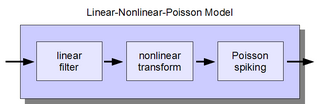
The linear-nonlinear-Poisson (LNP) cascade model is a simplified functional model of neural spike responses. It has been successfully used to describe the response characteristics of neurons in early sensory pathways, especially the visual system. The LNP model is generally implicit when using reverse correlation or the spike-triggered average to characterize neural responses with white-noise stimuli.
Spike-triggered covariance (STC) analysis is a tool for characterizing a neuron's response properties using the covariance of stimuli that elicit spikes from a neuron. STC is related to the spike-triggered average (STA), and provides a complementary tool for estimating linear filters in a linear-nonlinear-Poisson (LNP) cascade model. Unlike STA, the STC can be used to identify a multi-dimensional feature space in which a neuron computes its response.
In probability theory, the family of complex normal distributions, denoted or , characterizes complex random variables whose real and imaginary parts are jointly normal. The complex normal family has three parameters: location parameter μ, covariance matrix , and the relation matrix . The standard complex normal is the univariate distribution with , , and .
Linear least squares (LLS) is the least squares approximation of linear functions to data. It is a set of formulations for solving statistical problems involved in linear regression, including variants for ordinary (unweighted), weighted, and generalized (correlated) residuals. Numerical methods for linear least squares include inverting the matrix of the normal equations and orthogonal decomposition methods.
Maximally informative dimensions is a dimensionality reduction technique used in the statistical analyses of neural responses. Specifically, it is a way of projecting a stimulus onto a low-dimensional subspace so that as much information as possible about the stimulus is preserved in the neural response. It is motivated by the fact that natural stimuli are typically confined by their statistics to a lower-dimensional space than that spanned by white noise but correctly identifying this subspace using traditional techniques is complicated by the correlations that exist within natural images. Within this subspace, stimulus-response functions may be either linear or nonlinear. The idea was originally developed by Tatyana Sharpee, Nicole C. Rust, and William Bialek in 2003.
In the study of artificial neural networks (ANNs), the neural tangent kernel (NTK) is a kernel that describes the evolution of deep artificial neural networks during their training by gradient descent. It allows ANNs to be studied using theoretical tools from kernel methods.


