
In theoretical physics, a Feynman diagram is a pictorial representation of the mathematical expressions describing the behavior and interaction of subatomic particles. The scheme is named after American physicist Richard Feynman, who introduced the diagrams in 1948. The interaction of subatomic particles can be complex and difficult to understand; Feynman diagrams give a simple visualization of what would otherwise be an arcane and abstract formula. According to David Kaiser, "Since the middle of the 20th century, theoretical physicists have increasingly turned to this tool to help them undertake critical calculations. Feynman diagrams have revolutionized nearly every aspect of theoretical physics." While the diagrams are applied primarily to quantum field theory, they can also be used in other areas of physics, such as solid-state theory. Frank Wilczek wrote that the calculations that won him the 2004 Nobel Prize in Physics "would have been literally unthinkable without Feynman diagrams, as would [Wilczek's] calculations that established a route to production and observation of the Higgs particle."
In theoretical physics, quantum field theory (QFT) is a theoretical framework that combines classical field theory, special relativity, and quantum mechanics. QFT is used in particle physics to construct physical models of subatomic particles and in condensed matter physics to construct models of quasiparticles. The current standard model of particle physics is based on quantum field theory.
In physics, the screened Poisson equation is a Poisson equation, which arises in the Klein–Gordon equation, electric field screening in plasmas, and nonlocal granular fluidity in granular flow.
In theoretical physics, the term renormalization group (RG) refers to a formal apparatus that allows systematic investigation of the changes of a physical system as viewed at different scales. In particle physics, it reflects the changes in the underlying force laws as the energy scale at which physical processes occur varies, energy/momentum and resolution distance scales being effectively conjugate under the uncertainty principle.
In probability theory, the Borel–Kolmogorov paradox is a paradox relating to conditional probability with respect to an event of probability zero. It is named after Émile Borel and Andrey Kolmogorov.
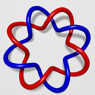
In mathematics, the linking number is a numerical invariant that describes the linking of two closed curves in three-dimensional space. Intuitively, the linking number represents the number of times that each curve winds around the other. In Euclidean space, the linking number is always an integer, but may be positive or negative depending on the orientation of the two curves.
In quantum mechanics and quantum field theory, the propagator is a function that specifies the probability amplitude for a particle to travel from one place to another in a given period of time, or to travel with a certain energy and momentum. In Feynman diagrams, which serve to calculate the rate of collisions in quantum field theory, virtual particles contribute their propagator to the rate of the scattering event described by the respective diagram. Propagators may also be viewed as the inverse of the wave operator appropriate to the particle, and are, therefore, often called (causal) Green's functions.
In quantum field theory, the quantum effective action is a modified expression for the classical action taking into account quantum corrections while ensuring that the principle of least action applies, meaning that extremizing the effective action yields the equations of motion for the vacuum expectation values of the quantum fields. The effective action also acts as a generating functional for one-particle irreducible correlation functions. The potential component of the effective action is called the effective potential, with the expectation value of the true vacuum being the minimum of this potential rather than the classical potential, making it important for studying spontaneous symmetry breaking.
In quantum field theory, a quartic interaction is a type of self-interaction in a scalar field. Other types of quartic interactions may be found under the topic of four-fermion interactions. A classical free scalar field satisfies the Klein–Gordon equation. If a scalar field is denoted , a quartic interaction is represented by adding a potential energy term to the Lagrangian density. The coupling constant is dimensionless in 4-dimensional spacetime.
In theoretical physics, dimensional regularization is a method introduced by Giambiagi and Bollini as well as – independently and more comprehensively – by 't Hooft and Veltman for regularizing integrals in the evaluation of Feynman diagrams; in other words, assigning values to them that are meromorphic functions of a complex parameter d, the analytic continuation of the number of spacetime dimensions.
In functional analysis, a branch of mathematics, it is sometimes possible to generalize the notion of the determinant of a square matrix of finite order (representing a linear transformation from a finite-dimensional vector space to itself) to the infinite-dimensional case of a linear operator S mapping a function space V to itself. The corresponding quantity det(S) is called the functional determinant of S.
In theoretical physics, a source is an abstract concept, developed by Julian Schwinger, motivated by the physical effects of surrounding particles involved in creating or destroying another particle. So, one can perceive sources as the origin of the physical properties carried by the created or destroyed particle, and thus one can use this concept to study all quantum processes including the spacetime localized properties and the energy forms, i.e., mass and momentum, of the phenomena. The probability amplitude of the created or the decaying particle is defined by the effect of the source on a localized spacetime region such that the affected particle captures its physics depending on the tensorial and spinorial nature of the source. An example that Julian Schwinger referred to is the creation of meson due to the mass correlations among five mesons.

Axial multipole moments are a series expansion of the electric potential of a charge distribution localized close to the origin along one Cartesian axis, denoted here as the z-axis. However, the axial multipole expansion can also be applied to any potential or field that varies inversely with the distance to the source, i.e., as . For clarity, we first illustrate the expansion for a single point charge, then generalize to an arbitrary charge density localized to the z-axis.
Cylindrical multipole moments are the coefficients in a series expansion of a potential that varies logarithmically with the distance to a source, i.e., as . Such potentials arise in the electric potential of long line charges, and the analogous sources for the magnetic potential and gravitational potential.
In theoretical physics, scalar field theory can refer to a relativistically invariant classical or quantum theory of scalar fields. A scalar field is invariant under any Lorentz transformation.
The Newman–Penrose (NP) formalism is a set of notation developed by Ezra T. Newman and Roger Penrose for general relativity (GR). Their notation is an effort to treat general relativity in terms of spinor notation, which introduces complex forms of the usual variables used in GR. The NP formalism is itself a special case of the tetrad formalism, where the tensors of the theory are projected onto a complete vector basis at each point in spacetime. Usually this vector basis is chosen to reflect some symmetry of the spacetime, leading to simplified expressions for physical observables. In the case of the NP formalism, the vector basis chosen is a null tetrad: a set of four null vectors—two real, and a complex-conjugate pair. The two real members often asymptotically point radially inward and radially outward, and the formalism is well adapted to treatment of the propagation of radiation in curved spacetime. The Weyl scalars, derived from the Weyl tensor, are often used. In particular, it can be shown that one of these scalars— in the appropriate frame—encodes the outgoing gravitational radiation of an asymptotically flat system.
The Frank–Tamm formula yields the amount of Cherenkov radiation emitted on a given frequency as a charged particle moves through a medium at superluminal velocity. It is named for Russian physicists Ilya Frank and Igor Tamm who developed the theory of the Cherenkov effect in 1937, for which they were awarded a Nobel Prize in Physics in 1958.
In the Newman–Penrose (NP) formalism of general relativity, independent components of the Ricci tensors of a four-dimensional spacetime are encoded into seven Ricci scalars which consist of three real scalars , three complex scalars and the NP curvature scalar . Physically, Ricci-NP scalars are related with the energy–momentum distribution of the spacetime due to Einstein's field equation.
In plasma physics and magnetic confinement fusion, neoclassical transport or neoclassical diffusion is a theoretical description of collisional transport in toroidal plasmas, usually found in tokamaks or stellarators. It is a modification of classical diffusion adding in effects of non-uniform magnetic fields due to the toroidal geometry, which give rise to new diffusion effects.
In theoretical physics, more specifically in quantum field theory and supersymmetry, supersymmetric Yang–Mills, also known as super Yang–Mills and abbreviated to SYM, is a supersymmetric generalization of Yang–Mills theory, which is a gauge theory that plays an important part in the mathematical formulation of forces in particle physics. It is a special case of 4D N = 1 global supersymmetry.


