Quadratic programming (QP) is the process of solving certain mathematical optimization problems involving quadratic functions. Specifically, one seeks to optimize a multivariate quadratic function subject to linear constraints on the variables. Quadratic programming is a type of nonlinear programming.
Mathematical optimization or mathematical programming is the selection of a best element, with regard to some criterion, from some set of available alternatives. It is generally divided into two subfields: discrete optimization and continuous optimization. Optimization problems arise in all quantitative disciplines from computer science and engineering to operations research and economics, and the development of solution methods has been of interest in mathematics for centuries.

Simulated annealing (SA) is a probabilistic technique for approximating the global optimum of a given function. Specifically, it is a metaheuristic to approximate global optimization in a large search space for an optimization problem. For large numbers of local optima, SA can find the global optima. It is often used when the search space is discrete. For problems where finding an approximate global optimum is more important than finding a precise local optimum in a fixed amount of time, simulated annealing may be preferable to exact algorithms such as gradient descent or branch and bound.
Gradient descent is a method for unconstrained mathematical optimization. It is a first-order iterative algorithm for finding a local minimum of a differentiable multivariate function.
Multi-disciplinary design optimization (MDO) is a field of engineering that uses optimization methods to solve design problems incorporating a number of disciplines. It is also known as multidisciplinary system design optimization (MSDO), and multidisciplinary design analysis and optimization (MDAO).
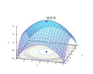
Global optimization is a branch of applied mathematics and numerical analysis that attempts to find the global minima or maxima of a function or a set of functions on a given set. It is usually described as a minimization problem because the maximization of the real-valued function is equivalent to the minimization of the function .
In mathematics, nonlinear programming (NLP) is the process of solving an optimization problem where some of the constraints or the objective function are nonlinear. An optimization problem is one of calculation of the extrema of an objective function over a set of unknown real variables and conditional to the satisfaction of a system of equalities and inequalities, collectively termed constraints. It is the sub-field of mathematical optimization that deals with problems that are not linear.
In optimization, line search is a basic iterative approach to find a local minimum of an objective function . It first finds a descent direction along which the objective function will be reduced, and then computes a step size that determines how far should move along that direction. The descent direction can be computed by various methods, such as gradient descent or quasi-Newton method. The step size can be determined either exactly or inexactly.
Boender-Rinnooy-Stougie-Timmer algorithm (BRST) is an optimization algorithm suitable for finding global optimum of black box functions. In their paper Boender et al. describe their method as a stochastic method involving a combination of sampling, clustering and local search, terminating with a range of confidence intervals on the value of the global minimum.
Covariance matrix adaptation evolution strategy (CMA-ES) is a particular kind of strategy for numerical optimization. Evolution strategies (ES) are stochastic, derivative-free methods for numerical optimization of non-linear or non-convex continuous optimization problems. They belong to the class of evolutionary algorithms and evolutionary computation. An evolutionary algorithm is broadly based on the principle of biological evolution, namely the repeated interplay of variation and selection: in each generation (iteration) new individuals are generated by variation, usually in a stochastic way, of the current parental individuals. Then, some individuals are selected to become the parents in the next generation based on their fitness or objective function value . Like this, over the generation sequence, individuals with better and better -values are generated.
Fitness approximation aims to approximate the objective or fitness functions in evolutionary optimization by building up machine learning models based on data collected from numerical simulations or physical experiments. The machine learning models for fitness approximation are also known as meta-models or surrogates, and evolutionary optimization based on approximated fitness evaluations are also known as surrogate-assisted evolutionary approximation. Fitness approximation in evolutionary optimization can be seen as a sub-area of data-driven evolutionary optimization.
Augmented Lagrangian methods are a certain class of algorithms for solving constrained optimization problems. They have similarities to penalty methods in that they replace a constrained optimization problem by a series of unconstrained problems and add a penalty term to the objective, but the augmented Lagrangian method adds yet another term designed to mimic a Lagrange multiplier. The augmented Lagrangian is related to, but not identical with, the method of Lagrange multipliers.
In computational engineering, Luus–Jaakola (LJ) denotes a heuristic for global optimization of a real-valued function. In engineering use, LJ is not an algorithm that terminates with an optimal solution; nor is it an iterative method that generates a sequence of points that converges to an optimal solution. However, when applied to a twice continuously differentiable function, the LJ heuristic is a proper iterative method, that generates a sequence that has a convergent subsequence; for this class of problems, Newton's method is recommended and enjoys a quadratic rate of convergence, while no convergence rate analysis has been given for the LJ heuristic. In practice, the LJ heuristic has been recommended for functions that need be neither convex nor differentiable nor locally Lipschitz: The LJ heuristic does not use a gradient or subgradient when one be available, which allows its application to non-differentiable and non-convex problems.

Adaptive coordinate descent is an improvement of the coordinate descent algorithm to non-separable optimization by the use of adaptive encoding. The adaptive coordinate descent approach gradually builds a transformation of the coordinate system such that the new coordinates are as decorrelated as possible with respect to the objective function. The adaptive coordinate descent was shown to be competitive to the state-of-the-art evolutionary algorithms and has the following invariance properties:
- Invariance with respect to monotonous transformations of the function (scaling)
- Invariance with respect to orthogonal transformations of the search space (rotation).
Bayesian optimization is a sequential design strategy for global optimization of black-box functions that does not assume any functional forms. It is usually employed to optimize expensive-to-evaluate functions.
Derivative-free optimization is a discipline in mathematical optimization that does not use derivative information in the classical sense to find optimal solutions: Sometimes information about the derivative of the objective function f is unavailable, unreliable or impractical to obtain. For example, f might be non-smooth, or time-consuming to evaluate, or in some way noisy, so that methods that rely on derivatives or approximate them via finite differences are of little use. The problem to find optimal points in such situations is referred to as derivative-free optimization, algorithms that do not use derivatives or finite differences are called derivative-free algorithms.
ANTIGONE, is a deterministic global optimization solver for general Mixed-Integer Nonlinear Programs (MINLP).
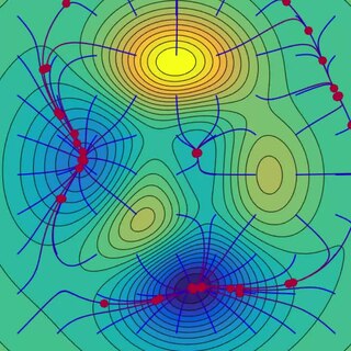
![Figure 1: MCS algorithm (without local search) applied to the two-dimensional Rosenbrock function. The global minimum
f
m
i
n
=
0
{\displaystyle f_{min}=0}
is located at
(
x
,
y
)
=
(
1
,
1
)
{\displaystyle (x,y)=(1,1)}
. MCS identifies a position with
f
[?]
0.002
{\displaystyle f\approx 0.002}
within 21 function evaluations. After additional 21 evaluations the optimal value is not improved and the algorithm terminates. Observe dense clustering of samples around potential minima - this effect can be reduced significantly by employing local searches appropriately. MCS algorithm.gif](http://upload.wikimedia.org/wikipedia/commons/thumb/d/d7/MCS_algorithm.gif/400px-MCS_algorithm.gif)


