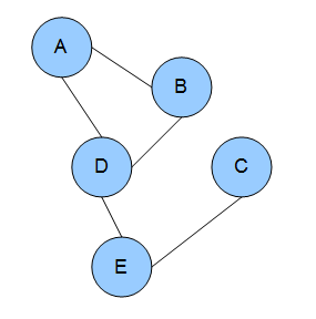
A Markov chain is a stochastic model describing a sequence of possible events in which the probability of each event depends only on the state attained in the previous event. A countably infinite sequence, in which the chain moves state at discrete time steps, gives a discrete-time Markov chain (DTMC). A continuous-time process is called a continuous-time Markov chain (CTMC). It is named after the Russian mathematician Andrey Markov.
Hidden Markov Model (HMM) is a statistical Markov model in which the system being modeled is assumed to be a Markov process – call it – with unobservable ("hidden") states. HMM assumes that there is another process whose behavior "depends" on . The goal is to learn about by observing . HMM stipulates that, for each time instance , the conditional probability distribution of given the history must not depend on .
Pattern recognition is the automated recognition of patterns and regularities in data. It has applications in statistical data analysis, signal processing, image analysis, information retrieval, bioinformatics, data compression, computer graphics and machine learning. Pattern recognition has its origins in statistics and engineering; some modern approaches to pattern recognition include the use of machine learning, due to the increased availability of big data and a new abundance of processing power. However, these activities can be viewed as two facets of the same field of application, and together they have undergone substantial development over the past few decades. A modern definition of pattern recognition is:
The field of pattern recognition is concerned with the automatic discovery of regularities in data through the use of computer algorithms and with the use of these regularities to take actions such as classifying the data into different categories.
A Bayesian network is a probabilistic graphical model that represents a set of variables and their conditional dependencies via a directed acyclic graph (DAG). Bayesian networks are ideal for taking an event that occurred and predicting the likelihood that any one of several possible known causes was the contributing factor. For example, a Bayesian network could represent the probabilistic relationships between diseases and symptoms. Given symptoms, the network can be used to compute the probabilities of the presence of various diseases.
The Viterbi algorithm is a dynamic programming algorithm for finding the most likely sequence of hidden states—called the Viterbi path—that results in a sequence of observed events, especially in the context of Markov information sources and hidden Markov models (HMM).

In probability theory and statistics, the term Markov property refers to the memoryless property of a stochastic process. It is named after the Russian mathematician Andrey Markov. The term strong Markov property is similar to the Markov property, except that the meaning of "present" is defined in terms of a random variable known as a stopping time.

In statistics, an expectation–maximization (EM) algorithm is an iterative method to find (local) maximum likelihood or maximum a posteriori (MAP) estimates of parameters in statistical models, where the model depends on unobserved latent variables. The EM iteration alternates between performing an expectation (E) step, which creates a function for the expectation of the log-likelihood evaluated using the current estimate for the parameters, and a maximization (M) step, which computes parameters maximizing the expected log-likelihood found on the E step. These parameter-estimates are then used to determine the distribution of the latent variables in the next E step.
In statistics, Gibbs sampling or a Gibbs sampler is a Markov chain Monte Carlo (MCMC) algorithm for obtaining a sequence of observations which are approximated from a specified multivariate probability distribution, when direct sampling is difficult. This sequence can be used to approximate the joint distribution ; to approximate the marginal distribution of one of the variables, or some subset of the variables ; or to compute an integral. Typically, some of the variables correspond to observations whose values are known, and hence do not need to be sampled.
In electrical engineering, computer science, statistical computing and bioinformatics, the Baum–Welch algorithm is a special case of the EM algorithm used to find the unknown parameters of a hidden Markov model (HMM). It makes use of the forward-backward algorithm to compute the statistics for the expectation step.
The forward algorithm, in the context of a hidden Markov model (HMM), is used to calculate a 'belief state': the probability of a state at a certain time, given the history of evidence. The process is also known as filtering. The forward algorithm is closely related to, but distinct from, the Viterbi algorithm.

In the domain of physics and probability, a Markov random field, Markov network or undirected graphical model is a set of random variables having a Markov property described by an undirected graph. In other words, a random field is said to be a Markov random field if it satisfies Markov properties.
A statistical language model is a probability distribution over sequences of words. Given such a sequence, say of length m, it assigns a probability to the whole sequence.
In Probability Theory, Statistics, and Machine Learning: Recursive Bayesian Estimation, also known as a Bayes Filter, is a general probabilistic approach for estimating an unknown probability density function (PDF) recursively over time using incoming measurements and a mathematical process model. The process relies heavily upon mathematical concepts and models that are theorized within a study of prior and posterior probabilities known as Bayesian Statistics.
Conditional random fields (CRFs) are a class of statistical modeling method often applied in pattern recognition and machine learning and used for structured prediction. Whereas a classifier predicts a label for a single sample without considering "neighboring" samples, a CRF can take context into account. To do so, the prediction is modeled as a graphical model, which implements dependencies between the predictions. What kind of graph is used depends on the application. For example, in natural language processing, linear chain CRFs are popular, which implement sequential dependencies in the predictions. In image processing the graph typically connects locations to nearby and/or similar locations to enforce that they receive similar predictions.
The forward–backward algorithm is an inference algorithm for hidden Markov models which computes the posterior marginals of all hidden state variables given a sequence of observations/emissions , i.e. it computes, for all hidden state variables , the distribution . This inference task is usually called smoothing. The algorithm makes use of the principle of dynamic programming to efficiently compute the values that are required to obtain the posterior marginal distributions in two passes. The first pass goes forward in time while the second goes backward in time; hence the name forward–backward algorithm.
The layered hidden Markov model (LHMM) is a statistical model derived from the hidden Markov model (HMM). A layered hidden Markov model (LHMM) consists of N levels of HMMs, where the HMMs on level i + 1 correspond to observation symbols or probability generators at level i. Every level i of the LHMM consists of Ki HMMs running in parallel.
In the mathematical theory of stochastic processes, variable-order Markov (VOM) models are an important class of models that extend the well known Markov chain models. In contrast to the Markov chain models, where each random variable in a sequence with a Markov property depends on a fixed number of random variables, in VOM models this number of conditioning random variables may vary based on the specific observed realization.
In the mathematical theory of probability, the entropy rate or source information rate of a stochastic process is, informally, the time density of the average information in a stochastic process. For stochastic processes with a countable index, the entropy rate is the limit of the joint entropy of members of the process divided by , as tends to infinity:
In machine learning, sequence labeling is a type of pattern recognition task that involves the algorithmic assignment of a categorical label to each member of a sequence of observed values. A common example of a sequence labeling task is part of speech tagging, which seeks to assign a part of speech to each word in an input sentence or document. Sequence labeling can be treated as a set of independent classification tasks, one per member of the sequence. However, accuracy is generally improved by making the optimal label for a given element dependent on the choices of nearby elements, using special algorithms to choose the globally best set of labels for the entire sequence at once.
In machine learning, the kernel embedding of distributions comprises a class of nonparametric methods in which a probability distribution is represented as an element of a reproducing kernel Hilbert space (RKHS). A generalization of the individual data-point feature mapping done in classical kernel methods, the embedding of distributions into infinite-dimensional feature spaces can preserve all of the statistical features of arbitrary distributions, while allowing one to compare and manipulate distributions using Hilbert space operations such as inner products, distances, projections, linear transformations, and spectral analysis. This learning framework is very general and can be applied to distributions over any space on which a sensible kernel function may be defined. For example, various kernels have been proposed for learning from data which are: vectors in , discrete classes/categories, strings, graphs/networks, images, time series, manifolds, dynamical systems, and other structured objects. The theory behind kernel embeddings of distributions has been primarily developed by Alex Smola, Le Song , Arthur Gretton, and Bernhard Schölkopf. A review of recent works on kernel embedding of distributions can be found in.


