Multinomial test

Last updated

Multinomial test is the statistical test of the null hypothesis that the parameters of a multinomial distribution equal specified values; it is used for categorical data. [1]

Beginning with a sample of items each of which has been observed to fall into one of categories. It is possible to define as the observed numbers of items in each cell. Hence

Next, defining a vector of parameters where: These are the parameter values under the null hypothesis.

The exact probability of the observed configuration under the null hypothesis is given by

The significance probability for the test is the probability of occurrence of the data set observed, or of a data set less likely than that observed, if the null hypothesis is true. Using an exact test, this is calculated as

where the sum ranges over all outcomes as likely as, or less likely than, that observed. In practice this becomes computationally onerous as and increase so it is probably only worth using exact tests for small samples. For larger samples, asymptotic approximations are accurate enough and easier to calculate.

One of these approximations is the likelihood ratio. An alternative hypothesis can be defined under which each value is replaced by its maximum likelihood estimate The exact probability of the observed configuration under the alternative hypothesis is given by

The natural logarithm of the likelihood ratio, between these two probabilities, multiplied by is then the statistic for the likelihood ratio test

(The factor is chosen to make the statistic asymptotically chi-squared distributed, for convenient comparison to a familiar statistic commonly used for the same application.)

If the null hypothesis is true, then as increases, the distribution of converges to that of chi-squared with degrees of freedom. However it has long been known (e.g. Lawley [2] ) that for finite sample sizes, the moments of are greater than those of chi-squared, thus inflating the probability of type I errors (false positives). The difference between the moments of chi-squared and those of the test statistic are a function of Williams [3] showed that the first moment can be matched as far as if the test statistic is divided by a factor given by

In the special case where the null hypothesis is that all the values are equal to (i.e. it stipulates a uniform distribution), this simplifies to

Subsequently, Smith et al. [4] derived a dividing factor which matches the first moment as far as For the case of equal values of this factor is

The null hypothesis can also be tested by using Pearson's chi-squared test

where is the expected number of cases in category under the null hypothesis. This statistic also converges to a chi-squared distribution with degrees of freedom when the null hypothesis is true but does so from below, as it were, rather than from above as does, so may be preferable to the uncorrected version of for small samples.[ citation needed ]

Related Research Articles

<span class="mw-page-title-main">Cauchy distribution</span> Probability distribution

The Cauchy distribution, named after Augustin Cauchy, is a continuous probability distribution. It is also known, especially among physicists, as the Lorentz distribution, Cauchy–Lorentz distribution, Lorentz(ian) function, or Breit–Wigner distribution. The Cauchy distribution is the distribution of the x-intercept of a ray issuing from with a uniformly distributed angle. It is also the distribution of the ratio of two independent normally distributed random variables with mean zero.

<span class="mw-page-title-main">Normal distribution</span> Probability distribution

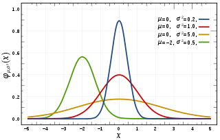
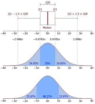
In probability theory and statistics, a normal distribution or Gaussian distribution is a type of continuous probability distribution for a real-valued random variable. The general form of its probability density function is The parameter is the mean or expectation of the distribution, while the parameter is the variance. The standard deviation of the distribution is . A random variable with a Gaussian distribution is said to be normally distributed, and is called a normal deviate.

<span class="mw-page-title-main">Probability density function</span> Concept in mathematics

In probability theory, a probability density function (PDF), density function, or density of an absolutely continuous random variable, is a function whose value at any given sample in the sample space can be interpreted as providing a relative likelihood that the value of the random variable would be equal to that sample. Probability density is the probability per unit length, in other words, while the absolute likelihood for a continuous random variable to take on any particular value is 0, the value of the PDF at two different samples can be used to infer, in any particular draw of the random variable, how much more likely it is that the random variable would be close to one sample compared to the other sample.

In statistics, the likelihood-ratio test is a hypothesis test that involves comparing the goodness of fit of two competing statistical models, typically one found by maximization over the entire parameter space and another found after imposing some constraint, based on the ratio of their likelihoods. If the more constrained model is supported by the observed data, the two likelihoods should not differ by more than sampling error. Thus the likelihood-ratio test tests whether this ratio is significantly different from one, or equivalently whether its natural logarithm is significantly different from zero.

<span class="mw-page-title-main">Multivariate normal distribution</span> Generalization of the one-dimensional normal distribution to higher dimensions

In probability theory and statistics, the multivariate normal distribution, multivariate Gaussian distribution, or joint normal distribution is a generalization of the one-dimensional (univariate) normal distribution to higher dimensions. One definition is that a random vector is said to be k-variate normally distributed if every linear combination of its k components has a univariate normal distribution. Its importance derives mainly from the multivariate central limit theorem. The multivariate normal distribution is often used to describe, at least approximately, any set of (possibly) correlated real-valued random variables, each of which clusters around a mean value.

<span class="mw-page-title-main">Student's t-distribution</span> Probability distribution

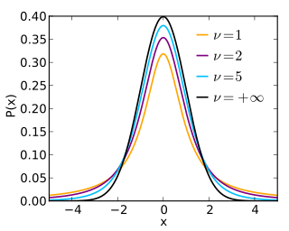
In probability and statistics, Student's t distribution is a continuous probability distribution that generalizes the standard normal distribution. Like the latter, it is symmetric around zero and bell-shaped.

In statistics, maximum likelihood estimation (MLE) is a method of estimating the parameters of an assumed probability distribution, given some observed data. This is achieved by maximizing a likelihood function so that, under the assumed statistical model, the observed data is most probable. The point in the parameter space that maximizes the likelihood function is called the maximum likelihood estimate. The logic of maximum likelihood is both intuitive and flexible, and as such the method has become a dominant means of statistical inference.

<span class="mw-page-title-main">Logistic regression</span> Statistical model for a binary dependent variable

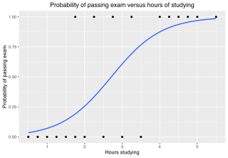
In statistics, the logistic model is a statistical model that models the log-odds of an event as a linear combination of one or more independent variables. In regression analysis, logistic regression estimates the parameters of a logistic model. In binary logistic regression there is a single binary dependent variable, coded by an indicator variable, where the two values are labeled "0" and "1", while the independent variables can each be a binary variable or a continuous variable. The corresponding probability of the value labeled "1" can vary between 0 and 1, hence the labeling; the function that converts log-odds to probability is the logistic function, hence the name. The unit of measurement for the log-odds scale is called a logit, from logistic unit, hence the alternative names. See § Background and § Definition for formal mathematics, and § Example for a worked example.

Pearson's chi-squared test or Pearson's test is a statistical test applied to sets of categorical data to evaluate how likely it is that any observed difference between the sets arose by chance. It is the most widely used of many chi-squared tests – statistical procedures whose results are evaluated by reference to the chi-squared distribution. Its properties were first investigated by Karl Pearson in 1900. In contexts where it is important to improve a distinction between the test statistic and its distribution, names similar to Pearson χ-squared test or statistic are used.

In statistics, the Wishart distribution is a generalization of the gamma distribution to multiple dimensions. It is named in honor of John Wishart, who first formulated the distribution in 1928. Other names include Wishart ensemble, or Wishart–Laguerre ensemble, or LOE, LUE, LSE.

In statistics, the score is the gradient of the log-likelihood function with respect to the parameter vector. Evaluated at a particular point of the parameter vector, the score indicates the steepness of the log-likelihood function and thereby the sensitivity to infinitesimal changes to the parameter values. If the log-likelihood function is continuous over the parameter space, the score will vanish at a local maximum or minimum; this fact is used in maximum likelihood estimation to find the parameter values that maximize the likelihood function.

In statistics, G-tests are likelihood-ratio or maximum likelihood statistical significance tests that are increasingly being used in situations where chi-squared tests were previously recommended.

Binomial test is an exact test of the statistical significance of deviations from a theoretically expected distribution of observations into two categories using sample data.

Variational Bayesian methods are a family of techniques for approximating intractable integrals arising in Bayesian inference and machine learning. They are typically used in complex statistical models consisting of observed variables as well as unknown parameters and latent variables, with various sorts of relationships among the three types of random variables, as might be described by a graphical model. As typical in Bayesian inference, the parameters and latent variables are grouped together as "unobserved variables". Variational Bayesian methods are primarily used for two purposes:

  1. To provide an analytical approximation to the posterior probability of the unobserved variables, in order to do statistical inference over these variables.
  2. To derive a lower bound for the marginal likelihood of the observed data. This is typically used for performing model selection, the general idea being that a higher marginal likelihood for a given model indicates a better fit of the data by that model and hence a greater probability that the model in question was the one that generated the data.

Estimation theory is a branch of statistics that deals with estimating the values of parameters based on measured empirical data that has a random component. The parameters describe an underlying physical setting in such a way that their value affects the distribution of the measured data. An estimator attempts to approximate the unknown parameters using the measurements. In estimation theory, two approaches are generally considered:

In statistics, the Bayesian information criterion (BIC) or Schwarz information criterion is a criterion for model selection among a finite set of models; models with lower BIC are generally preferred. It is based, in part, on the likelihood function and it is closely related to the Akaike information criterion (AIC).

A ratio distribution is a probability distribution constructed as the distribution of the ratio of random variables having two other known distributions. Given two random variables X and Y, the distribution of the random variable Z that is formed as the ratio Z = X/Y is a ratio distribution.

In probability theory, the family of complex normal distributions, denoted or , characterizes complex random variables whose real and imaginary parts are jointly normal. The complex normal family has three parameters: location parameter μ, covariance matrix , and the relation matrix . The standard complex normal is the univariate distribution with , , and .

In statistics, Wilks' theorem offers an asymptotic distribution of the log-likelihood ratio statistic, which can be used to produce confidence intervals for maximum-likelihood estimates or as a test statistic for performing the likelihood-ratio test.

In machine learning, the kernel embedding of distributions comprises a class of nonparametric methods in which a probability distribution is represented as an element of a reproducing kernel Hilbert space (RKHS). A generalization of the individual data-point feature mapping done in classical kernel methods, the embedding of distributions into infinite-dimensional feature spaces can preserve all of the statistical features of arbitrary distributions, while allowing one to compare and manipulate distributions using Hilbert space operations such as inner products, distances, projections, linear transformations, and spectral analysis. This learning framework is very general and can be applied to distributions over any space on which a sensible kernel function may be defined. For example, various kernels have been proposed for learning from data which are: vectors in , discrete classes/categories, strings, graphs/networks, images, time series, manifolds, dynamical systems, and other structured objects. The theory behind kernel embeddings of distributions has been primarily developed by Alex Smola, Le Song , Arthur Gretton, and Bernhard Schölkopf. A review of recent works on kernel embedding of distributions can be found in.

References

  1. Read, T.R.C.; Cressie, N.A.C. (1988). Goodness-of-Fit Statistics for Discrete Multivariate Data. New York, NY: Springer-Verlag. ISBN   0-387-96682-X.
  2. Lawley, D.N. (1956). "A general method of approximating to the distribution of likelihood ratio criteria". Biometrika. 43: 295–303. doi:10.1093/biomet/43.3-4.295.
  3. Williams, D.A. (1976). "Improved Likelihood Ratio Tests for Complete Contingency Tables". Biometrika. 63: 33–37. doi:10.1093/biomet/63.1.33.
  4. Smith, P.J.; Rae, D.S.; Manderscheid, R.W.; Manderscheid, S. (1981). "Approximating the moments and distribution of the likelihood ratio statistic for multinomial goodness of fit". Journal of the American Statistical Association. 76 (375). American Statistical Association: 737–740. doi:10.2307/2287541. JSTOR   2287541.