Multiple factor analysis

Last updated

Multiple factor analysis (MFA) is a factorial method [1] devoted to the study of tables in which a group of individuals is described by a set of variables (quantitative and / or qualitative) structured in groups. It is a multivariate method from the field of ordination used to simplify multidimensional data structures. MFA treats all involved tables in the same way (symmetrical analysis). It may be seen as an extension of:

Contents

Introductory example

Why introduce several active groups of variables in the same factorial analysis?

data

Consider the case of quantitative variables, that is to say, within the framework of the PCA. An example of data from ecological research provides a useful illustration. There are, for 72 stations, two types of measurements:

  1. The abundance-dominance coefficient of 50 plant species (coefficient ranging from 0 = the plant is absent, to 9 = the species covers more than three-quarters of the surface). The whole set of the 50 coefficients defines the floristic profile of a station.
  2. Eleven pedological measurements (Pedology = soil science): particle size, physical, chemistry, etc. The set of these eleven measures defines the pedological profile of a station.

Three analyses are possible:

  1. PCA of flora (pedology as supplementary): this analysis focuses on the variability of the floristic profiles. Two stations are close one another if they have similar floristic profiles. In a second step, the main dimensions of this variability (i.e. the principal components) are related to the pedological variables introduced as supplementary.
  2. PCA of pedology (flora as supplementary): this analysis focuses on the variability of soil profiles. Two stations are close if they have the same soil profile. The main dimensions of this variability (i.e. the principal components) are then related to the abundance of plants.
  3. PCA of the two groups of variables as active: one may want to study the variability of stations from both the point of view of flora and soil. In this approach, two stations should be close if they have both similar flora 'and' similar soils.

Balance between groups of variables

Methodology

The third analysis of the introductory example implicitly assumes a balance between flora and soil. However, in this example, the mere fact that the flora is represented by 50 variables and the soil by 11 variables implies that the PCA with 61 active variables will be influenced mainly by the flora at least on the first axis). This is not desirable: there is no reason to wish one group play a more important role in the analysis.

The core of MFA is based on a factorial analysis (PCA in the case of quantitative variables, MCA in the case of qualitative variables) in which the variables are weighted. These weights are identical for the variables of the same group (and vary from one group to another). They are such that the maximum axial inertia of a group is equal to 1: in other words, by applying the PCA (or, where applicable, the MCA) to one group with this weighting, we obtain a first eigenvalue equal to 1. To get this property, MFA assigns to each variable of group a weight equal to the inverse of the first eigenvalue of the analysis (PCA or MCA according to the type of variable) of the group .

Formally, noting the first eigenvalue of the factorial analysis of one group , the MFA assigns weight for each variable of the group .

Balancing maximum axial inertia rather than the total inertia (= the number of variables in standard PCA) gives the MFA several important properties for the user. More directly, its interest appears in the following example.

Example

Let two groups of variables defined on the same set of individuals.

  1. Group 1 is composed of two uncorrelated variables A and B.
  2. Group 2 is composed of two variables {C1, C2} identical to the same variable C uncorrelated with the first two.

This example is not completely unrealistic. It is often necessary to simultaneously analyse multi-dimensional and (quite) one-dimensional groups.

Each group having the same number of variables has the same total inertia.

In this example the first axis of the PCA is almost coincident with C. Indeed, in the space of variables, there are two variables in the direction of C: group 2, with all its inertia concentrated in one direction, influences predominantly the first axis. For its part, group 1, consisting of two orthogonal variables (= uncorrelated), has its inertia uniformly distributed in a plane (the plane generated by the two variables) and hardly weighs on the first axis.

Numerical Example

Table 1. MFA. Test data. A and B (group 1) are uncorrelated. C1 and C2 (group 2) are identical.
1111
2344
3522
4522
5344
6122
Table 2. Test data. Decomposition of the inertia in the PCA and in the MFA applied to data in Table 1.
PCA
Inertia2.14 (100%)1
group 10.24(11%)1
group 21.91(89%)0
MFA
Inertia1.28(100%)1
group 10.64(50%)1
group 20.64(50%)0

Table 2 summarizes the inertia of the first two axes of the PCA and of the MFA applied to Table 1.

Group 2 variables contribute to 88.95% of the inertia of the axis 1 of the PCA. The first axis () is almost coincident with C: the correlation between C and is .976;

The first axis of the MFA (on Table 1 data) shows the balance between the two groups of variables: the contribution of each group to the inertia of this axis is strictly equal to 50%.

The second axis, meanwhile, depends only on group 1. This is natural since this group is two-dimensional while the second group, being one-dimensional, can be highly related to only one axis (here the first axis).

Conclusion about the balance between groups

Introducing several active groups of variables in a factorial analysis implicitly assumes a balance between these groups.

This balance must take into account that a multidimensional group influences naturally more axes than a one-dimensional group does (which may not be closely related to one axis).

The weighting of the MFA, which makes the maximum axial inertia of each group equal to 1, plays this role.

Application examples

Survey Questionnaires are always structured according to different themes. Each theme is a group of variables, for example, questions about opinions and questions about behaviour. Thus, in this example, we may want to perform a factorial analysis in which two individuals are close if they have both expressed the same opinions and the same behaviour.

Sensory analysis A same set of products has been evaluated by a panel of experts and a panel of consumers. For its evaluation, each jury uses a list of descriptors (sour, bitter, etc.). Each judge scores each descriptor for each product on a scale of intensity ranging for example from 0 = null or very low to 10 = very strong. In the table associated with a jury, at the intersection of the row and column , is the average score assigned to product for descriptor .

Individuals are the products. Each jury is a group of variables. We want to achieve a factorial analysis in which two products are similar if they were evaluated in the same way by both juries.

Multidimensional time series variables are measured on individuals. These measurements are made at dates. There are many ways to analyse such data set. One way suggested by MFA is to consider each day as a group of variables in the analysis of the tables (each table corresponds to one date) juxtaposed row-wise (the table analysed thus has rows and x columns).

Conclusion: These examples show that in practice, variables are very often organized into groups.

Graphics from MFA

Beyond the weighting of variables, interest in MFA lies in a series of graphics and indicators valuable in the analysis of a table whose columns are organized into groups.

Graphics common to all the simple factorial analyses (PCA, MCA)

The core of MFA is a weighted factorial analysis: MFA firstly provides the classical results of the factorial analyses.

1. Representations of individuals in which two individuals are close to each other if they exhibit similar values for many variables in the different variable groups; in practice the user particularly studies the first factorial plane.

2.Representations of quantitative variables as in PCA (correlation circle).

Figure1. MFA. Test data. Representation of individuals on the first plane. AFM fig1.jpg
Figure1. MFA. Test data. Representation of individuals on the first plane.
Figure2. MFA. Test data. Representation of variables on the first plane. AFM fig2.jpg
Figure2. MFA. Test data. Representation of variables on the first plane.

In the example:

3. Indicators aiding interpretation: projected inertia, contributions and quality of representation. In the example, the contribution of individuals 1 and 5 to the inertia of the first axis is 45.7% + 31.5% = 77.2% which justifies the interpretation focussed on these two points.

4. Representations of categories of qualitative variables as in MCA (a category lies at the centroid of the individuals who possess it). No qualitative variables in the example.

Graphics specific to this kind of multiple table

5. Superimposed representations of individuals « seen » by each group. An individual considered from the point of view of a single group is called partial individual (in parallel, an individual considered from the point of view of all variables is said mean individual because it lies at the center of gravity of its partial points). Partial cloud gathers the individuals from the perspective of the single group (ie ): that is the cloud analysed in the separate factorial analysis (PCA or MCA) of the group . The superimposed representation of the provided by the MFA is similar in its purpose to that provided by the Procrustes analysis.

Figure 3. MFA. Test data. Superimposed representation of mean and partial clouds. AFM fig3.jpg
Figure 3. MFA. Test data. Superimposed representation of mean and partial clouds.

In the example (figure 3), individual 1 is characterized by a small size (i.e. small values) both in terms of group 1 and group 2 (partial points of the individual 1 have a negative coordinate and are close one another). On the contrary, the individual 5 is more characterized by high values for the variables of group 2 than for the variables of group 1 (for the individual 5, group 2 partial point lies further from the origin than group 1 partial point). This reading of the graph can be checked directly in the data.

6. Representations of groups of variables as such. In these graphs, each group of variables is represented by a single point. Two groups of variables are close one another when they define the same structure on individuals. Extreme case: two groups of variables that define homothetic clouds of individuals coincide. The coordinate of group along the axis is equal to the contribution of the group to the inertia of MFA dimension of rank . This contribution can be interpreted as an indicator of relationship (between the group and the axis , hence the name relationship square given to this type of representation). This representation also exists in other factorial methods (MCA and FAMD in particular) in which case the groups of variable are each reduced to a single variable.

Figure4. MFA. Test data. Representation of groups of variables. AFM fig4.jpg
Figure4. MFA. Test data. Representation of groups of variables.

In the example (Figure 4), this representation shows that the first axis is related to the two groups of variables, while the second axis is related to the first group. This agrees with the representation of the variables (figure 2). In practice, this representation is especially precious when the groups are numerous and include many variables.

Other reading grid. The two groups of variables have in common the size effect (first axis) and differ according to axis 2 since this axis is specific to group 1 (he opposes the variables A and B).

7. Representations of factors of separate analyses of the different groups. These factors are represented as supplementary quantitative variables (correlation circle).

Figure 5. MFA. Test data. Representation of the principal components of separate PCA of each group. AFM fig5.jpg
Figure 5. MFA. Test data. Representation of the principal components of separate PCA of each group.

In the example (figure 5), the first axis of the MFA is relatively strongly correlated (r = .80) to the first component of the group 2. This group, consisting of two identical variables, possesses only one principal component (confounded with the variable). The group 1 consists of two orthogonal variables: any direction of the subspace generated by these two variables has the same inertia (equal to 1). So there is uncertainty in the choice of principal components and there is no reason to be interested in one of them in particular. However, the two components provided by the program are well represented: the plane of the MFA is close to the plane spanned by the two variables of group 1.

Conclusion

The numerical example illustrates the output of the MFA. Besides balancing groups of variables and besides usual graphics of PCA (of MCA in the case of qualitative variables), the MFA provides results specific of the group structure of the set of variables, that is, in particular:

The small size and simplicity of the example allow simple validation of the rules of interpretation. But the method will be more valuable when the data set is large and complex. Other methods suitable for this type of data are available. Procrustes analysis is compared to the MFA in. [2]

History

MFA was developed by Brigitte Escofier and Jérôme Pagès in the 1980s. It is at the heart of two books written by these authors: [3] and. [4] The MFA and its extensions (hierarchical MFA, MFA on contingency tables, etc.) are a research topic of applied mathematics laboratory Agrocampus (LMA ²) which published a book presenting basic methods of exploratory multivariate analysis. [5]

Software

MFA is available in two R packages (FactoMineR and ADE4) and in many software packages, including SPAD, Uniwin, XLSTAT, etc. There is also a function SAS [ permanent dead link ] . The graphs in this article come from the R package FactoMineR.

Related Research Articles

Analysis of variance (ANOVA) is a collection of statistical models and their associated estimation procedures used to analyze the differences among means. ANOVA was developed by the statistician Ronald Fisher. ANOVA is based on the law of total variance, where the observed variance in a particular variable is partitioned into components attributable to different sources of variation. In its simplest form, ANOVA provides a statistical test of whether two or more population means are equal, and therefore generalizes the t-test beyond two means. In other words, the ANOVA is used to test the difference between two or more means.

<span class="mw-page-title-main">Principal component analysis</span> Method of data analysis

Principal component analysis (PCA) is a linear dimensionality reduction technique with applications in exploratory data analysis, visualization and data preprocessing.

Factor analysis is a statistical method used to describe variability among observed, correlated variables in terms of a potentially lower number of unobserved variables called factors. For example, it is possible that variations in six observed variables mainly reflect the variations in two unobserved (underlying) variables. Factor analysis searches for such joint variations in response to unobserved latent variables. The observed variables are modelled as linear combinations of the potential factors plus "error" terms, hence factor analysis can be thought of as a special case of errors-in-variables models.

<span class="mw-page-title-main">Social research</span> Research conducted by social scientists

Social research is research conducted by social scientists following a systematic plan. Social research methodologies can be classified as quantitative and qualitative.

<span class="mw-page-title-main">Quantitative research</span> All procedures for the numerical representation of empirical facts

Quantitative research is a research strategy that focuses on quantifying the collection and analysis of data. It is formed from a deductive approach where emphasis is placed on the testing of theory, shaped by empiricist and positivist philosophies.

Survival analysis is a branch of statistics for analyzing the expected duration of time until one event occurs, such as death in biological organisms and failure in mechanical systems. This topic is called reliability theory or reliability analysis in engineering, duration analysis or duration modelling in economics, and event history analysis in sociology. Survival analysis attempts to answer certain questions, such as what is the proportion of a population which will survive past a certain time? Of those that survive, at what rate will they die or fail? Can multiple causes of death or failure be taken into account? How do particular circumstances or characteristics increase or decrease the probability of survival?

<span class="mw-page-title-main">Interaction (statistics)</span> Statistical term

In statistics, an interaction may arise when considering the relationship among three or more variables, and describes a situation in which the effect of one causal variable on an outcome depends on the state of a second causal variable. Although commonly thought of in terms of causal relationships, the concept of an interaction can also describe non-causal associations. Interactions are often considered in the context of regression analyses or factorial experiments.

<span class="mw-page-title-main">Economic model</span> Simplified representation of economic reality

An economic model is a theoretical construct representing economic processes by a set of variables and a set of logical and/or quantitative relationships between them. The economic model is a simplified, often mathematical, framework designed to illustrate complex processes. Frequently, economic models posit structural parameters. A model may have various exogenous variables, and those variables may change to create various responses by economic variables. Methodological uses of models include investigation, theorizing, and fitting theories to the world.

In statistics, a categorical variable is a variable that can take on one of a limited, and usually fixed, number of possible values, assigning each individual or other unit of observation to a particular group or nominal category on the basis of some qualitative property. In computer science and some branches of mathematics, categorical variables are referred to as enumerations or enumerated types. Commonly, each of the possible values of a categorical variable is referred to as a level. The probability distribution associated with a random categorical variable is called a categorical distribution.

In group theory, a branch of abstract algebra, a character table is a two-dimensional table whose rows correspond to irreducible representations, and whose columns correspond to conjugacy classes of group elements. The entries consist of characters, the traces of the matrices representing group elements of the column's class in the given row's group representation. In chemistry, crystallography, and spectroscopy, character tables of point groups are used to classify e.g. molecular vibrations according to their symmetry, and to predict whether a transition between two states is forbidden for symmetry reasons. Many university level textbooks on physical chemistry, quantum chemistry, spectroscopy and inorganic chemistry devote a chapter to the use of symmetry group character tables.

Linear discriminant analysis (LDA), normal discriminant analysis (NDA), or discriminant function analysis is a generalization of Fisher's linear discriminant, a method used in statistics and other fields, to find a linear combination of features that characterizes or separates two or more classes of objects or events. The resulting combination may be used as a linear classifier, or, more commonly, for dimensionality reduction before later classification.

<span class="mw-page-title-main">Factorial experiment</span> Experimental design in statistics

In statistics, a full factorial experiment is an experiment whose design consists of two or more factors, each with discrete possible values or "levels", and whose experimental units take on all possible combinations of these levels across all such factors. A full factorial design may also be called a fully crossed design. Such an experiment allows the investigator to study the effect of each factor on the response variable, as well as the effects of interactions between factors on the response variable.

This glossary of statistics and probability is a list of definitions of terms and concepts used in the mathematical sciences of statistics and probability, their sub-disciplines, and related fields. For additional related terms, see Glossary of mathematics and Glossary of experimental design.

In statistics, the frequency or absolute frequency of an event is the number of times the observation has occurred/recorded in an experiment or study. These frequencies are often depicted graphically or in tabular form.

Correspondence analysis (CA) is a multivariate statistical technique proposed by Herman Otto Hartley (Hirschfeld) and later developed by Jean-Paul Benzécri. It is conceptually similar to principal component analysis, but applies to categorical rather than continuous data. In a similar manner to principal component analysis, it provides a means of displaying or summarising a set of data in two-dimensional graphical form. Its aim is to display in a biplot any structure hidden in the multivariate setting of the data table. As such it is a technique from the field of multivariate ordination. Since the variant of CA described here can be applied either with a focus on the rows or on the columns it should in fact be called simple (symmetric) correspondence analysis.

<span class="mw-page-title-main">Plot (graphics)</span> Graphical technique for data sets

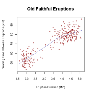
A plot is a graphical technique for representing a data set, usually as a graph showing the relationship between two or more variables. The plot can be drawn by hand or by a computer. In the past, sometimes mechanical or electronic plotters were used. Graphs are a visual representation of the relationship between variables, which are very useful for humans who can then quickly derive an understanding which may not have come from lists of values. Given a scale or ruler, graphs can also be used to read off the value of an unknown variable plotted as a function of a known one, but this can also be done with data presented in tabular form. Graphs of functions are used in mathematics, sciences, engineering, technology, finance, and other areas.

In statistics, multiple correspondence analysis (MCA) is a data analysis technique for nominal categorical data, used to detect and represent underlying structures in a data set. It does this by representing data as points in a low-dimensional Euclidean space. The procedure thus appears to be the counterpart of principal component analysis for categorical data. MCA can be viewed as an extension of simple correspondence analysis (CA) in that it is applicable to a large set of categorical variables.

In statistics, factor analysis of mixed data or factorial analysis of mixed data, is the factorial method devoted to data tables in which a group of individuals is described both by quantitative and qualitative variables. It belongs to the exploratory methods developed by the French school called Analyse des données founded by Jean-Paul Benzécri.

In statistics, the relationship square is a graphical representation for use in the factorial analysis of a table individuals x variables. This representation completes classical representations provided by principal component analysis (PCA) or multiple correspondence analysis (MCA), namely those of individuals, of quantitative variables and of the categories of qualitative variables. It is especially important in factor analysis of mixed data (FAMD) and in multiple factor analysis (MFA).

References

  1. Greenacre, Michael; Blasius, Jorg (2006-06-23). Multiple Correspondence Analysis and Related Methods. CRC Press. pp. 352–. ISBN   9781420011319 . Retrieved 11 June 2014.
  2. Pagès Jérôme (2014). Multiple Factor Analysis by Example Using R. Chapman & Hall/CRC The R Series, London. 272p
  3. Ibidem
  4. Escofier Brigitte & Pagès Jérôme (2008). Analyses factorielles simples et multiples; objectifs, méthodes et interprétation. Dunod, Paris. 318 p. ISBN   978-2-10-051932-3
  5. Husson F., Lê S. & Pagès J. (2009). Exploratory Multivariate Analysis by Example Using R. Chapman & Hall/CRC The R Series, London. ISBN   978-2-7535-0938-2