
The quantum harmonic oscillator is the quantum-mechanical analog of the classical harmonic oscillator. Because an arbitrary smooth potential can usually be approximated as a harmonic potential at the vicinity of a stable equilibrium point, it is one of the most important model systems in quantum mechanics. Furthermore, it is one of the few quantum-mechanical systems for which an exact, analytical solution is known.
In quantum mechanics, a density matrix is a matrix that describes the quantum state of a physical system. It allows for the calculation of the probabilities of the outcomes of any measurement performed upon this system, using the Born rule. It is a generalization of the more usual state vectors or wavefunctions: while those can only represent pure states, density matrices can also represent mixed states. Mixed states arise in quantum mechanics in two different situations:
- when the preparation of the system is not fully known, and thus one must deal with a statistical ensemble of possible preparations, and
- when one wants to describe a physical system that is entangled with another, without describing their combined state; this case is typical for a system interacting with some environment.

Quantum decoherence is the loss of quantum coherence, the process in which a system's behaviour changes from that which can be explained by quantum mechanics to that which can be explained by classical mechanics. In quantum mechanics, particles such as electrons are described by a wave function, a mathematical representation of the quantum state of a system; a probabilistic interpretation of the wave function is used to explain various quantum effects. As long as there exists a definite phase relation between different states, the system is said to be coherent. A definite phase relationship is necessary to perform quantum computing on quantum information encoded in quantum states. Coherence is preserved under the laws of quantum physics.
In physics, specifically in quantum mechanics, a coherent state is the specific quantum state of the quantum harmonic oscillator, often described as a state that has dynamics most closely resembling the oscillatory behavior of a classical harmonic oscillator. It was the first example of quantum dynamics when Erwin Schrödinger derived it in 1926, while searching for solutions of the Schrödinger equation that satisfy the correspondence principle. The quantum harmonic oscillator arise in the quantum theory of a wide range of physical systems. For instance, a coherent state describes the oscillating motion of a particle confined in a quadratic potential well. The coherent state describes a state in a system for which the ground-state wavepacket is displaced from the origin of the system. This state can be related to classical solutions by a particle oscillating with an amplitude equivalent to the displacement.
In quantum mechanics, the Gorini–Kossakowski–Sudarshan–Lindblad equation, master equation in Lindblad form, quantum Liouvillian, or Lindbladian is one of the general forms of Markovian master equations describing open quantum systems. It generalizes the Schrödinger equation to open quantum systems; that is, systems in contacts with their surroundings. The resulting dynamics is no longer unitary, but still satisfies the property of being trace-preserving and completely positive for any initial condition.
A quasiprobability distribution is a mathematical object similar to a probability distribution but which relaxes some of Kolmogorov's axioms of probability theory. Quasiprobabilities share several of general features with ordinary probabilities, such as, crucially, the ability to yield expectation values with respect to the weights of the distribution. However, they can violate the σ-additivity axiom: integrating over them does not necessarily yield probabilities of mutually exclusive states. Indeed, quasiprobability distributions also have regions of negative probability density, counterintuitively, contradicting the first axiom. Quasiprobability distributions arise naturally in the study of quantum mechanics when treated in phase space formulation, commonly used in quantum optics, time-frequency analysis, and elsewhere.
The Glauber–Sudarshan P representation is a suggested way of writing down the phase space distribution of a quantum system in the phase space formulation of quantum mechanics. The P representation is the quasiprobability distribution in which observables are expressed in normal order. In quantum optics, this representation, formally equivalent to several other representations, is sometimes preferred over such alternative representations to describe light in optical phase space, because typical optical observables, such as the particle number operator, are naturally expressed in normal order. It is named after George Sudarshan and Roy J. Glauber, who worked on the topic in 1963. Despite many useful applications in laser theory and coherence theory, the Sudarshan–Glauber P representation has the peculiarity that it is not always positive, and is not a bona-fide probability function.
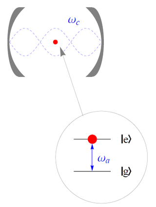
The Jaynes–Cummings model is a theoretical model in quantum optics. It describes the system of a two-level atom interacting with a quantized mode of an optical cavity, with or without the presence of light. It was originally developed to study the interaction of atoms with the quantized electromagnetic field in order to investigate the phenomena of spontaneous emission and absorption of photons in a cavity.
In many-body theory, the term Green's function is sometimes used interchangeably with correlation function, but refers specifically to correlators of field operators or creation and annihilation operators.
In physics, a quantum amplifier is an amplifier that uses quantum mechanical methods to amplify a signal; examples include the active elements of lasers and optical amplifiers.

The Husimi Q representation, introduced by Kôdi Husimi in 1940, is a quasiprobability distribution commonly used in quantum mechanics to represent the phase space distribution of a quantum state such as light in the phase space formulation. It is used in the field of quantum optics and particularly for tomographic purposes. It is also applied in the study of quantum effects in superconductors.
An electric dipole transition is the dominant effect of an interaction of an electron in an atom with the electromagnetic field.
The phase-space formulation of quantum mechanics places the position and momentum variables on equal footing in phase space. In contrast, the Schrödinger picture uses the position or momentum representations. The two key features of the phase-space formulation are that the quantum state is described by a quasiprobability distribution and operator multiplication is replaced by a star product.
Coherent states are quasi-classical states that may be defined in different ways, for instance as eigenstates of the annihilation operator
Quantum stochastic calculus is a generalization of stochastic calculus to noncommuting variables. The tools provided by quantum stochastic calculus are of great use for modeling the random evolution of systems undergoing measurement, as in quantum trajectories. Just as the Lindblad master equation provides a quantum generalization to the Fokker–Planck equation, quantum stochastic calculus allows for the derivation of quantum stochastic differential equations (QSDE) that are analogous to classical Langevin equations.
A quantum heat engine is a device that generates power from the heat flow between hot and cold reservoirs. The operation mechanism of the engine can be described by the laws of quantum mechanics. The first realization of a quantum heat engine was pointed out by Scovil and Schulz-DuBois in 1959, showing the connection of efficiency of the Carnot engine and the 3-level maser. Quantum refrigerators share the structure of quantum heat engines with the purpose of pumping heat from a cold to a hot bath consuming power first suggested by Geusic, Schulz-DuBois, De Grasse and Scovil. When the power is supplied by a laser the process is termed optical pumping or laser cooling, suggested by Wineland and Hänsch. Surprisingly heat engines and refrigerators can operate up to the scale of a single particle thus justifying the need for a quantum theory termed quantum thermodynamics.

Quantum thermodynamics is the study of the relations between two independent physical theories: thermodynamics and quantum mechanics. The two independent theories address the physical phenomena of light and matter. In 1905, Albert Einstein argued that the requirement of consistency between thermodynamics and electromagnetism leads to the conclusion that light is quantized, obtaining the relation . This paper is the dawn of quantum theory. In a few decades quantum theory became established with an independent set of rules. Currently quantum thermodynamics addresses the emergence of thermodynamic laws from quantum mechanics. It differs from quantum statistical mechanics in the emphasis on dynamical processes out of equilibrium. In addition, there is a quest for the theory to be relevant for a single individual quantum system.
In quantum probability, the Belavkin equation, also known as Belavkin-Schrödinger equation, quantum filtering equation, stochastic master equation, is a quantum stochastic differential equation describing the dynamics of a quantum system undergoing observation in continuous time. It was derived and henceforth studied by Viacheslav Belavkin in 1988.
Hamiltonian truncation is a numerical method used to study quantum field theories (QFTs) in spacetime dimensions. Hamiltonian truncation is an adaptation of the Rayleigh–Ritz method from quantum mechanics. It is closely related to the exact diagonalization method used to treat spin systems in condensed matter physics. The method is typically used to study QFTs on spacetimes of the form , specifically to compute the spectrum of the Hamiltonian along . A key feature of Hamiltonian truncation is that an explicit ultraviolet cutoff is introduced, akin to the lattice spacing a in lattice Monte Carlo methods. Since Hamiltonian truncation is a nonperturbative method, it can be used to study strong-coupling phenomena like spontaneous symmetry breaking.
In lattice field theory, the Wilson action is a discrete formulation of the Yang–Mills action, forming the foundation of lattice gauge theory. Rather than using Lie algebra valued gauge fields as the fundamental parameters of the theory, group valued link fields are used instead, which correspond to the smallest Wilson lines on the lattice. In modern simulations of pure gauge theory, the action is usually modified by introducing higher order operators through Symanzik improvement, significantly reducing discretization errors. The action was introduced by Kenneth Wilson in his seminal 1974 paper, launching the study of lattice field theory.


