Coherence is defined as the ability of waves to interfere. Intuitively, coherent waves have a well-defined constant phase relationship. However, an exclusive and extensive physical definition of coherence is more nuanced. Coherence functions, as introduced by Roy Glauber and others in the 1960s, capture the mathematics behind the intuition by defining correlation between the electric field components as coherence.[1] These correlations between electric field components can be measured to arbitrary orders, hence leading to the concept of different orders of coherence.[2] The coherence encountered in most optical experiments, including the classic Young's double slit experiment and Mach–Zehnder interferometer, is first order coherence. Robert Hanbury Brown and Richard Q. Twiss performed a correlation experiment in 1956, and brought to light a different kind of correlation between fields, namely the correlation of intensities, which correspond to second order coherence.[3] Higher order coherences become relevant in photon-coincidence counting experiments.[4] Orders of coherence can be measured using classical correlation functions or by using the quantum analogue of those functions, which take quantum mechanical description of electric field (operators) as input. While the quantum coherence functions might yield the same results as the classical functions, the underlying mechanism and description of the physical processes are fundamentally different because quantum interference deals with interference of possible histories while classical interference deals with interference of physical waves.[1]
The electric field can be separated into its positive and negative frequency components . Either of the two frequency components, contains all the physical information about the wave.[1] The classical first-order, second order and nth order correlation function are defined as follows
,
,
,
where represents . While the order of the and , does not matter in the classical case, as they are merely numbers and hence commute, the ordering is vital in the quantum analogue of these correlation functions.[2] The first order correlation function, measured at the same time and position gives us the intensity i.e. . The classical nth order normalized correlation function is defined by dividing the nth order correlation function by all corresponding intensities: .
In quantum mechanics, the positive and negative frequency components of the electric field are replaced by the operators and respectively. In the Heisenberg picture, , where is the polarization vector, is the unit vector perpendicular to , with signifying one of the two vectors that are perpedincular to the polarization vector, is the frequency of the mode and is the volume.[3] The nth order quantum correlation function is defined as:
.
Here the orders of the and operators do matter. This is because the positive and the negative frequency ( and ) components are proportional the annhiliation and the creation operators respectively, and and do not commute. When the operators are written in the order shown in the equation above, they are said to be in a normal ordering. Subsequently, the nth order normalized correlation function is defined as:
.
A field is said to m-coherent if the mth normalized correlation function is unity. This definition holds for both and .
Young double slit experiment
Figure 1. Schematic diagram for the setup of the Young's Double Slit Experiment.
In Young's double slit experiment, light from a light source is allowed to pass through two pinholes separated by some distance, and a screen is placed some distance away from the pinholes where the interference between the light waves is observed (Figure. 1). Young's double slit experiment demonstrates the dependence of interference on coherence, specifically on the first-order correlation. This experiment is equivalent to the Mach–Zehnder interferometer with the caveat that Young's double slit experiment is concerned with spatial coherence, while the Mach–Zehnder interferometer relies on temporal coherence.[2]
The intensity measured at the position at time is
.
Light field has highest degree of coherence when the corresponding interference pattern has the maximum contrast on the screen. The fringe contrast is defined as .
Classically, and hence . As coherence is the ability to interfere visibility and coherence are linked:
means highest contrast, complete coherence
means partial fringe visibility, partial coherence
Classically, the electric field at a position , is the sum of electric field components from at the two pinholes and earlier times respectably i.e. . Correspondingly, in the quantum description the electric field operators are similarly related, . This implies
.
The intensity fluctuates as a function of position i.e. the quantum mechanical treatment also predicts interference fringes. Moreover, in accordance to the intuitive understanding of coherence i.e. ability to interfere, the interference patterns depend on the first-order correlation function .[1] Comparing this to the classical intensity, we note that the only difference is that the classical normalized correlation is now replaced by the quantum correlation . Even the computations here look strikingly similar to the ones that might be done classically.[2] However, the quantum interference that occurs in this process is fundamentally different from the classical interference of electromagnetic waves. Quantum interference occurs when two possible histories, given a particular initial and final state, interfere. In this experiment, given an initial state of the photon before the pinhole and it final state at the screen, the two possible histories correspond to the two pinholes through which the photon could have passed. Hence, quantum mechanically, here the photon is interfering with itself. Such interference of different histories, however, occurs only when the observer has no specific way of determining which of the different histories actually occurred. If the system is observed to determine the path of the photon, then on average the interference of amplitudes will vanish.[1]
Hanbury Brown and Twiss experiment
Figure 2. A schematic diagram for the setup for Hanbury Brown and Twiss's original experiment.
In the Hanbury Brown and Twiss experiment (Figure 2.), a light beam is split using a beam splitter and then detected by detectors, which are equidistant from the beam splitter. Subsequently, signal measured by the second detector is delayed by time and the coincidence rate between the original and delayed signal is counted. This experiment correlates intensities, , rather than electric fields and hence measures the second order correlation function
.
Under the assumption of stationary statistics, at a given position, the normalized correlation function is
here measures the probability of coincidence of two photons being detected with a time difference .[2]
For all varieties of chaotic light, the following relationship between the first order and second-order coherences holds:
.
This relationship is true for both the classical and quantum correlation functions. Moreover, as always takes a value between 0 and 1, for a chaotic light beam, . The light source used by Hanbury Brown and Twiss was stellar light which is chaotic. Hanbury Brown and Twiss used this result to compute the first order coherence from their measurement of the second order coherence. The observed second order coherence the curve was as shown in figure 2.[5]
For Gaussian light source . Often a Gaussian light source is chaotic and consequently,
Figure 3. The second order coherence for stellar light as measured in the Hanbury Brown and Twiss experiment as a function of the time delay introduced between the signals , where is the coherence length.
.
This model fits the observation that was done by Hanbury Brown and Twiss using stellar light as demonstrated in figure 3. If thermal light was used instead of stellar light in the same setup, then we would see a different function for the second order coherence.[5] Thermal light can be modeled to be a Lorentzian power spectrum centered around frequency , which means , where is the coherence length of the beam. Correspondingly, and . The second-order coherence for stellar (Gaussian), thermal (Lorentzian) and coherent light is shown in Figure 4. Note that when stellar/thermal light beam is first order coherent i.e. , the second order coherence is 2, meaning at zero time delay chaotic light right is first order coherent but not second order coherent.[3][5]
Quantum description
Classically, we can think of a light beam as having a probability distribution as a function of mode amplitudes, and in that case, the second order correlation function . If we assume that the quantum state of the setup is , then the quantum mechanical correlation function,, which is same as the classical result.[6]
Figure 4. The second order coherence for thermal, stellar and coherent light as a function of time delay. is the coherence length of the light beam.
Similar to the case of Young's double slit experiment, the classical and the quantum description lead to the same result, but that does not mean that two descriptions are equivalent. Classically, the light beams arrives as an electromagnetic wave and interferes owing to the superposition principle. The quantum description is not as straightforward. To understand the subtleties in the quantum description, assume that photons from the source are emitted independent of each other at the source and that the photons are not split by the beam splitter. When the intensity of the source is set to be very low, such that only one photon might be detected at any time, accounting for the fact that there might be accidental coincidences, which are statistically independent of time, the coincidence counter should not change with respect to the time difference. However, as shown in Figure 3., for stellar light , so without any time delay and with a large time delay . Hence, even when there was no time-delay the photons from the source were arriving in pairs! This effect is termed photon bunching. Moreover, if a laser light was used at the source instead of chaotic light, then second order coherence would be independent of the time delay. HBT's experiment allows for a fundamentally distinction in the way in which photons are emitted from a laser compared to a natural light source. Such a distinction is not captured by the classical description on wave interference.[1]
Higher-order coherences and mathematical properties of coherence functions
For the purposes of standard optical experiments, coherence is just first-order coherence and higher-order coherences are generally ignored. Higher order coherences are measured in photon-coincidence counting experiments. Correlation interferometry uses coherences of fourth-order and higher to perform stellar measurements.[4][7] We can think of as the average coincidence rate of detecting photons at positions.[3] Physically, these rate are always positive and therefore .
mth order coherent fields
A field is called mth order coherent if there exists a function such that all correlation functions for factorize. Notationally, this means
This factorizability of all correlation functions implies that . As was defined to be , it follows that for , if the field is m-coherent.[7] For a m-coherent field, the photons being detected will be detected statistically independent of each other.[1]
Upper bound the order of coherence
Given an upper bound on how many photons can be present in the field, there is an upper bound on the Mth coherence the field can have. This is because is proportional the annihilation operator. To see this, begin with a mixed state for the field . If this sum has an upper limit on n, m i.e. , is proportional to for . This result would be unintuitive in a classical description, but fortunately such a case has no classical counterpart because we cannot put an upper bound on the number of photons in the classical case.[1]
Stationarity of the statistics
When dealing with classical optics, physicists often employ the assumption that the statistics of the system are stationary. This means that while the observations might fluctuate, the underlying statistics of the system remains constant as time progresses. The quantum analogue of stationary statistics is to require that the density operator, which contains the information about the wavefunction, commutes with the Hamiltonian. Owing to Schrödinger equation, , stationary statistics implies that the density operator is independent of time. Consequently, in, owing to the cyclicity of the trace, we can transform the time independence of the density operator in the Schrödinger picture to the time independence of and , in the Heisenberg picture, giving us
.
This means that under the assumption that the underlying statistics of the system are stationary, the nth order correlation functions do not change when every time argument is translated by the same amount. In other words, rather than looking at actual times, the correlation function is only concerned with the time differences.[1]
Coherent states
Coherent state are quantum mechanical states that have the maximal coherence and have the most "classical"-like behavior. A coherent state is defined as the quantum mechanical state that is the eigenstate of the electric field operator . As is directly proportional to the annihilation operator the coherent state is an eigenstate of the annihilation operator. Given a coherent state , . Consequently, coherent states have all orders of coherences as being non-zero.[8]
In mechanics, the virial theorem provides a general equation that relates the average over time of the total kinetic energy of a stable system of discrete particles, bound by potential forces, with that of the total potential energy of the system. Mathematically, the theorem states
In physics, a Langevin equation is a stochastic differential equation describing how a system evolves when subjected to a combination of deterministic and fluctuating ("random") forces. The dependent variables in a Langevin equation typically are collective (macroscopic) variables changing only slowly in comparison to the other (microscopic) variables of the system. The fast (microscopic) variables are responsible for the stochastic nature of the Langevin equation. One application is to Brownian motion, which models the fluctuating motion of a small particle in a fluid.
In physics, specifically in quantum mechanics, a coherent state is the specific quantum state of the quantum harmonic oscillator, often described as a state which has dynamics most closely resembling the oscillatory behavior of a classical harmonic oscillator. It was the first example of quantum dynamics when Erwin Schrödinger derived it in 1926, while searching for solutions of the Schrödinger equation that satisfy the correspondence principle. The quantum harmonic oscillator arise in the quantum theory of a wide range of physical systems. For instance, a coherent state describes the oscillating motion of a particle confined in a quadratic potential well. The coherent state describes a state in a system for which the ground-state wavepacket is displaced from the origin of the system. This state can be related to classical solutions by a particle oscillating with an amplitude equivalent to the displacement.
An instanton is a notion appearing in theoretical and mathematical physics. An instanton is a classical solution to equations of motion with a finite, non-zero action, either in quantum mechanics or in quantum field theory. More precisely, it is a solution to the equations of motion of the classical field theory on a Euclidean spacetime.
The Drude model of electrical conduction was proposed in 1900 by Paul Drude to explain the transport properties of electrons in materials. Basically, Ohm's law was well established and stated that the current J and voltage V driving the current are related to the resistance R of the material. The inverse of the resistance is known as the conductance. When we consider a metal of unit length and unit cross sectional area, the conductance is known as the conductivity, which is the inverse of resistivity. The Drude model attempts to explain the resistivity of a conductor in terms of the scattering of electrons by the relatively immobile ions in the metal that act like obstructions to the flow of electrons.
The adiabatic theorem is a concept in quantum mechanics. Its original form, due to Max Born and Vladimir Fock (1928), was stated as follows:
In physics, the Hanbury Brown and Twiss (HBT) effect is any of a variety of correlation and anti-correlation effects in the intensities received by two detectors from a beam of particles. HBT effects can generally be attributed to the wave–particle duality of the beam, and the results of a given experiment depend on whether the beam is composed of fermions or bosons. Devices which use the effect are commonly called intensity interferometers and were originally used in astronomy, although they are also heavily used in the field of quantum optics.
In statistical mechanics, the correlation function is a measure of the order in a system, as characterized by a mathematical correlation function. Correlation functions describe how microscopic variables, such as spin and density, at different positions are related. More specifically, correlation functions quantify how microscopic variables co-vary with one another on average across space and time. A classic example of such spatial correlations is in ferro- and antiferromagnetic materials, where the spins prefer to align parallel and antiparallel with their nearest neighbors, respectively. The spatial correlation between spins in such materials is shown in the figure to the right.
In quantum optics, correlation functions are used to characterize the statistical and coherence properties of an electromagnetic field. The degree of coherence is the normalized correlation of electric fields; in its simplest form, termed . It is useful for quantifying the coherence between two electric fields, as measured in a Michelson or other linear optical interferometer. The correlation between pairs of fields, , typically is used to find the statistical character of intensity fluctuations. First order correlation is actually the amplitude-amplitude correlation and the second order correlation is the intensity-intensity correlation. It is also used to differentiate between states of light that require a quantum mechanical description and those for which classical fields are sufficient. Analogous considerations apply to any Bose field in subatomic physics, in particular to mesons.
Quantum noise is noise arising from the indeterminate state of matter in accordance with fundamental principles of quantum mechanics, specifically the uncertainty principle and via zero-point energy fluctuations. Quantum noise is due to the apparently discrete nature of the small quantum constituents such as electrons, as well as the discrete nature of quantum effects, such as photocurrents.
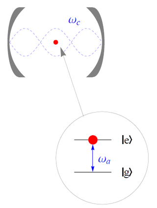
The Jaynes–Cummings model is a theoretical model in quantum optics. It describes the system of a two-level atom interacting with a quantized mode of an optical cavity, with or without the presence of light. It was originally developed to study the interaction of atoms with the quantized electromagnetic field in order to investigate the phenomena of spontaneous emission and absorption of photons in a cavity.
The theoretical and experimental justification for the Schrödinger equation motivates the discovery of the Schrödinger equation, the equation that describes the dynamics of nonrelativistic particles. The motivation uses photons, which are relativistic particles with dynamics described by Maxwell's equations, as an analogue for all types of particles.
In many-body theory, the term Green's function is sometimes used interchangeably with correlation function, but refers specifically to correlators of field operators or creation and annihilation operators.
Resonance fluorescence is the process in which a two-level atom system interacts with the quantum electromagnetic field if the field is driven at a frequency near to the natural frequency of the atom.
Photon antibunching generally refers to a light field with photons more equally spaced than a coherent laser field, a signature being signals at appropriate detectors which are anticorrelated. More specifically, it can refer to sub-Poissonian photon statistics, that is a photon number distribution for which the variance is less than the mean. A coherent state, as output by a laser far above threshold, has Poissonian statistics yielding random photon spacing; while a thermal light field has super-Poissonian statistics and yields bunched photon spacing. In the thermal (bunched) case, the number of fluctuations is larger than a coherent state; for an antibunched source they are smaller.
In statistical mechanics, the Griffiths inequality, sometimes also called Griffiths–Kelly–Sherman inequality or GKS inequality, named after Robert B. Griffiths, is a correlation inequality for ferromagnetic spin systems. Informally, it says that in ferromagnetic spin systems, if the 'a-priori distribution' of the spin is invariant under spin flipping, the correlation of any monomial of the spins is non-negative; and the two point correlation of two monomial of the spins is non-negative.
The semiconductor luminescence equations (SLEs) describe luminescence of semiconductors resulting from spontaneous recombination of electronic excitations, producing a flux of spontaneously emitted light. This description established the first step toward semiconductor quantum optics because the SLEs simultaneously includes the quantized light–matter interaction and the Coulomb-interaction coupling among electronic excitations within a semiconductor. The SLEs are one of the most accurate methods to describe light emission in semiconductors and they are suited for a systematic modeling of semiconductor emission ranging from excitonic luminescence to lasers.
The Mandel Q parameter measures the departure of the occupation number distribution from Poissonian statistics. It was introduced in quantum optics by Leonard Mandel. It is a convenient way to characterize non-classical states with negative values indicating a sub-Poissonian statistics, which have no classical analog. It is defined as the normalized variance of the boson distribution:
Magnetic resonance is a quantum mechanical resonant effect that can appear when a magnetic dipole is exposed to a static magnetic field and perturbed with another, oscillating electromagnetic field. Due to the static field, the dipole can assume a number of discrete energy eigenstates, depending on the value of its angular momentum quantum number. The oscillating field can then make the dipole transit between its energy states with a certain probability and at a certain rate. The overall transition probability will depend on the field's frequency and the rate will depend on its amplitude. When the frequency of that field leads to the maximum possible transition probability between two states, a magnetic resonance has been achieved. In that case, the energy of the photons composing the oscillating field matches the energy difference between said states. If the dipole is tickled with a field oscillating far from resonance, it is unlikely to transition. That is analogous to other resonant effects, such as with the forced harmonic oscillator. The periodic transition between the different states is called Rabi cycle and the rate at which that happens is called Rabi frequency. The Rabi frequency should not be confused with the field's own frequency. Since many atomic nuclei species can behave as a magnetic dipole, this resonance technique is the basis of nuclear magnetic resonance, including nuclear magnetic resonance imaging and nuclear magnetic resonance spectroscopy.
In this article spherical functions are replaced by polynomials that have been well known in electrostatics since the time of Maxwell and associated with multipole moments. In physics, dipole and quadrupole moments typically appear because fundamental concepts of physics are associated precisely with them. Dipole and quadrupole moments are:
↑ Deutsch, Ivan (November 12, 2015). "Lectures on Quantum Optics"(PDF). Interferometry and coherence: Hanbury Brown and Twiss. University of New Mexico. Retrieved December 10, 2015.
This page is based on this Wikipedia article Text is available under the CC BY-SA 4.0 license; additional terms may apply. Images, videos and audio are available under their respective licenses.