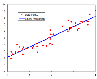
The method of least squares is a standard approach in regression analysis to approximate the solution of overdetermined systems by minimizing the sum of the squares of the residuals made in the results of each individual equation.

In statistical modeling, regression analysis is a set of statistical processes for estimating the relationships between a dependent variable and one or more independent variables. The most common form of regression analysis is linear regression, in which one finds the line that most closely fits the data according to a specific mathematical criterion. For example, the method of ordinary least squares computes the unique line that minimizes the sum of squared differences between the true data and that line. For specific mathematical reasons, this allows the researcher to estimate the conditional expectation of the dependent variable when the independent variables take on a given set of values. Less common forms of regression use slightly different procedures to estimate alternative location parameters or estimate the conditional expectation across a broader collection of non-linear models.

In applied statistics, total least squares is a type of errors-in-variables regression, a least squares data modeling technique in which observational errors on both dependent and independent variables are taken into account. It is a generalization of Deming regression and also of orthogonal regression, and can be applied to both linear and non-linear models.

In statistics, nonlinear regression is a form of regression analysis in which observational data are modeled by a function which is a nonlinear combination of the model parameters and depends on one or more independent variables. The data are fitted by a method of successive approximations.
In statistics, multicollinearity is a phenomenon in which one predictor variable in a multiple regression model can be linearly predicted from the others with a substantial degree of accuracy. In this situation, the coefficient estimates of the multiple regression may change erratically in response to small changes in the model or the data. Multicollinearity does not reduce the predictive power or reliability of the model as a whole, at least within the sample data set; it only affects calculations regarding individual predictors. That is, a multivariable regression model with collinear predictors can indicate how well the entire bundle of predictors predicts the outcome variable, but it may not give valid results about any individual predictor, or about which predictors are redundant with respect to others.

In statistics, the coefficient of determination, denoted R2 or r2 and pronounced "R squared", is the proportion of the variation in the dependent variable that is predictable from the independent variable(s).
In statistics, ordinary least squares (OLS) is a type of linear least squares method for choosing the unknown parameters in a linear regression model by the principle of least squares: minimizing the sum of the squares of the differences between the observed dependent variable in the input dataset and the output of the (linear) function of the independent variable.
In statistics, the Breusch–Pagan test, developed in 1979 by Trevor Breusch and Adrian Pagan, is used to test for heteroskedasticity in a linear regression model. It was independently suggested with some extension by R. Dennis Cook and Sanford Weisberg in 1983. Derived from the Lagrange multiplier test principle, it tests whether the variance of the errors from a regression is dependent on the values of the independent variables. In that case, heteroskedasticity is present.
In statistics, Mallows's Cp, named for Colin Lingwood Mallows, is used to assess the fit of a regression model that has been estimated using ordinary least squares. It is applied in the context of model selection, where a number of predictor variables are available for predicting some outcome, and the goal is to find the best model involving a subset of these predictors. A small value of Cp means that the model is relatively precise.
In statistics, the projection matrix, sometimes also called the influence matrix or hat matrix, maps the vector of response values to the vector of fitted values. It describes the influence each response value has on each fitted value. The diagonal elements of the projection matrix are the leverages, which describe the influence each response value has on the fitted value for that same observation.
In statistics, regression validation is the process of deciding whether the numerical results quantifying hypothesized relationships between variables, obtained from regression analysis, are acceptable as descriptions of the data. The validation process can involve analyzing the goodness of fit of the regression, analyzing whether the regression residuals are random, and checking whether the model's predictive performance deteriorates substantially when applied to data that were not used in model estimation.
In linear regression, mean response and predicted response are values of the dependent variable calculated from the regression parameters and a given value of the independent variable. The values of these two responses are the same, but their calculated variances are different.
In applied statistics, a partial regression plot attempts to show the effect of adding another variable to a model that already has one or more independent variables. Partial regression plots are also referred to as added variable plots, adjusted variable plots, and individual coefficient plots.
In regression analysis, partial leverage (PL) is a measure of the contribution of the individual independent variables to the total leverage of each observation. That is, if hi is the ith element of the diagonal of the hat matrix, PL is a measure of how hi changes as a variable is added to the regression model. It is computed as:
In statistics and in particular in regression analysis, leverage is a measure of how far away the independent variable values of an observation are from those of the other observations. High-leverage points, if any, are outliers with respect to the independent variables. That is, high-leverage points have no neighboring points in space, where is the number of independent variables in a regression model. This makes the fitted model likely to pass close to a high leverage observation. Hence high-leverage points have the potential to cause large changes in the parameter estimates when they are deleted i.e., to be influential points. Although an influential point will typically have high leverage, a high leverage point is not necessarily an influential point. The leverage is typically defined as the diagonal elements of the hat matrix.
In statistics, polynomial regression is a form of regression analysis in which the relationship between the independent variable x and the dependent variable y is modelled as an nth degree polynomial in x. Polynomial regression fits a nonlinear relationship between the value of x and the corresponding conditional mean of y, denoted E(y |x). Although polynomial regression fits a nonlinear model to the data, as a statistical estimation problem it is linear, in the sense that the regression function E(y | x) is linear in the unknown parameters that are estimated from the data. For this reason, polynomial regression is considered to be a special case of multiple linear regression.
In statistics, projection pursuit regression (PPR) is a statistical model developed by Jerome H. Friedman and Werner Stuetzle which is an extension of additive models. This model adapts the additive models in that it first projects the data matrix of explanatory variables in the optimal direction before applying smoothing functions to these explanatory variables.
Linear least squares (LLS) is the least squares approximation of linear functions to data. It is a set of formulations for solving statistical problems involved in linear regression, including variants for ordinary (unweighted), weighted, and generalized (correlated) residuals. Numerical methods for linear least squares include inverting the matrix of the normal equations and orthogonal decomposition methods.
In statistics, the variance function is a smooth function which depicts the variance of a random quantity as a function of its mean. The variance function is a measure of heteroscedasticity and plays a large role in many settings of statistical modelling. It is a main ingredient in the generalized linear model framework and a tool used in non-parametric regression, semiparametric regression and functional data analysis. In parametric modeling, variance functions take on a parametric form and explicitly describe the relationship between the variance and the mean of a random quantity. In a non-parametric setting, the variance function is assumed to be a smooth function.
In statistics, linear regression is a linear approach for modelling the relationship between a scalar response and one or more explanatory variables. The case of one explanatory variable is called simple linear regression; for more than one, the process is called multiple linear regression. This term is distinct from multivariate linear regression, where multiple correlated dependent variables are predicted, rather than a single scalar variable.


