
In regression analysis, least squares is a parameter estimation method based on minimizing the sum of the squares of the residuals made in the results of each individual equation.

Poisson's equation is an elliptic partial differential equation of broad utility in theoretical physics. For example, the solution to Poisson's equation is the potential field caused by a given electric charge or mass density distribution; with the potential field known, one can then calculate the corresponding electrostatic or gravitational (force) field. It is a generalization of Laplace's equation, which is also frequently seen in physics. The equation is named after French mathematician and physicist Siméon Denis Poisson who published it in 1823.
In probability theory and statistics, the Zipf–Mandelbrot law is a discrete probability distribution. Also known as the Pareto–Zipf law, it is a power-law distribution on ranked data, named after the linguist George Kingsley Zipf, who suggested a simpler distribution called Zipf's law, and the mathematician Benoit Mandelbrot, who subsequently generalized it.

The unified neutral theory of biodiversity and biogeography is a theory and the title of a monograph by ecologist Stephen P. Hubbell. It aims to explain the diversity and relative abundance of species in ecological communities. Like other neutral theories of ecology, Hubbell assumes that the differences between members of an ecological community of trophically similar species are "neutral", or irrelevant to their success. This implies that niche differences do not influence abundance and the abundance of each species follows a random walk. The theory has sparked controversy, and some authors consider it a more complex version of other null models that fit the data better.
In statistics, a generalized linear model (GLM) is a flexible generalization of ordinary linear regression. The GLM generalizes linear regression by allowing the linear model to be related to the response variable via a link function and by allowing the magnitude of the variance of each measurement to be a function of its predicted value.
In statistics, a mixture model is a probabilistic model for representing the presence of subpopulations within an overall population, without requiring that an observed data set should identify the sub-population to which an individual observation belongs. Formally a mixture model corresponds to the mixture distribution that represents the probability distribution of observations in the overall population. However, while problems associated with "mixture distributions" relate to deriving the properties of the overall population from those of the sub-populations, "mixture models" are used to make statistical inferences about the properties of the sub-populations given only observations on the pooled population, without sub-population identity information. Mixture models are used for clustering, under the name model-based clustering, and also for density estimation.
Spatial ecology studies the ultimate distributional or spatial unit occupied by a species. In a particular habitat shared by several species, each of the species is usually confined to its own microhabitat or spatial niche because two species in the same general territory cannot usually occupy the same ecological niche for any significant length of time.
A paleothermometer is a methodology that provides an estimate of the ambient temperature at the time of formation of a natural material. Most paleothermometers are based on empirically-calibrated proxy relationships, such as the tree ring or TEX86 methods. Isotope methods, such as the δ18O method or the clumped-isotope method, are able to provide, at least in theory, direct measurements of temperature.
In statistics, Poisson regression is a generalized linear model form of regression analysis used to model count data and contingency tables. Poisson regression assumes the response variable Y has a Poisson distribution, and assumes the logarithm of its expected value can be modeled by a linear combination of unknown parameters. A Poisson regression model is sometimes known as a log-linear model, especially when used to model contingency tables.
Phytogeography or botanical geography is the branch of biogeography that is concerned with the geographic distribution of plant species and their influence on the earth's surface. Phytogeography is concerned with all aspects of plant distribution, from the controls on the distribution of individual species ranges to the factors that govern the composition of entire communities and floras. Geobotany, by contrast, focuses on the geographic space's influence on plants.
In statistics, binomial regression is a regression analysis technique in which the response has a binomial distribution: it is the number of successes in a series of independent Bernoulli trials, where each trial has probability of success . In binomial regression, the probability of a success is related to explanatory variables: the corresponding concept in ordinary regression is to relate the mean value of the unobserved response to explanatory variables.
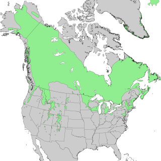
Species distribution, or speciesdispersion, is the manner in which a biological taxon is spatially arranged. The geographic limits of a particular taxon's distribution is its range, often represented as shaded areas on a map. Patterns of distribution change depending on the scale at which they are viewed, from the arrangement of individuals within a small family unit, to patterns within a population, or the distribution of the entire species as a whole (range). Species distribution is not to be confused with dispersal, which is the movement of individuals away from their region of origin or from a population center of high density.

In ecology, local abundance is the relative representation of a species in a particular ecosystem. It is usually measured as the number of individuals found per sample. The ratio of abundance of one species to one or multiple other species living in an ecosystem is referred to as relative species abundances. Both indicators are relevant for computing biodiversity.
In spatial ecology and macroecology, scaling pattern of occupancy (SPO), also known as the area-of-occupancy (AOO) is the way in which species distribution changes across spatial scales. In physical geography and image analysis, it is similar to the modifiable areal unit problem. Simon A. Levin (1992) states that the problem of relating phenomena across scales is the central problem in biology and in all of science. Understanding the SPO is thus one central theme in ecology.
Mechanistic models for niche apportionment are biological models used to explain relative species abundance distributions. These niche apportionment models describe how species break up resource pool in multi-dimensional space, determining the distribution of abundances of individuals among species. The relative abundances of species are usually expressed as a Whittaker plot, or rank abundance plot, where species are ranked by number of individuals on the x-axis, plotted against the log relative abundance of each species on the y-axis. The relative abundance can be measured as the relative number of individuals within species or the relative biomass of individuals within species.
Relative species abundance is a component of biodiversity and is a measure of how common or rare a species is relative to other species in a defined location or community. Relative abundance is the percent composition of an organism of a particular kind relative to the total number of organisms in the area. Relative species abundances tend to conform to specific patterns that are among the best-known and most-studied patterns in macroecology. Different populations in a community exist in relative proportions; this idea is known as relative abundance.
The generalized Lotka–Volterra equations are a set of equations which are more general than either the competitive or predator–prey examples of Lotka–Volterra types. They can be used to model direct competition and trophic relationships between an arbitrary number of species. Their dynamics can be analysed analytically to some extent. This makes them useful as a theoretical tool for modeling food webs. However, they lack features of other ecological models such as predator preference and nonlinear functional responses, and they cannot be used to model mutualism without allowing indefinite population growth.

Species distribution modelling (SDM), also known as environmental(or ecological) niche modelling (ENM), habitat modelling, predictive habitat distribution modelling, and range mapping uses ecological models to predict the distribution of a species across geographic space and time using environmental data. The environmental data are most often climate data (e.g. temperature, precipitation), but can include other variables such as soil type, water depth, and land cover. SDMs are used in several research areas in conservation biology, ecology and evolution. These models can be used to understand how environmental conditions influence the occurrence or abundance of a species, and for predictive purposes (ecological forecasting). Predictions from an SDM may be of a species’ future distribution under climate change, a species’ past distribution in order to assess evolutionary relationships, or the potential future distribution of an invasive species. Predictions of current and/or future habitat suitability can be useful for management applications (e.g. reintroduction or translocation of vulnerable species, reserve placement in anticipation of climate change).
Taylor's power law is an empirical law in ecology that relates the variance of the number of individuals of a species per unit area of habitat to the corresponding mean by a power law relationship. It is named after the ecologist who first proposed it in 1961, Lionel Roy Taylor (1924–2007). Taylor's original name for this relationship was the law of the mean. The name Taylor's law was coined by Southwood in 1966.
In statistics, the class of vector generalized linear models (VGLMs) was proposed to enlarge the scope of models catered for by generalized linear models (GLMs). In particular, VGLMs allow for response variables outside the classical exponential family and for more than one parameter. Each parameter can be transformed by a link function. The VGLM framework is also large enough to naturally accommodate multiple responses; these are several independent responses each coming from a particular statistical distribution with possibly different parameter values.


