Proportional control

Last updated July 23, 2022

Proportional control, in engineering and process control, is a type of linear feedback control system in which a correction is applied to the controlled variable, and the size of the correction is proportional to the difference between the desired value (setpoint, SP) and the measured value (process variable, PV). Two classic mechanical examples are the toilet bowl float proportioning valve and the fly-ball governor.

The proportional control concept is more complex than an on–off control system such as a bi-metallic domestic thermostat, but simpler than a proportional–integral–derivative (PID) control system used in something like an automobile cruise control. On–off control will work where the overall system has a relatively long response time, but can result in instability if the system being controlled has a rapid response time. Proportional control overcomes this by modulating the output to the controlling device, such as a control valve at a level which avoids instability, but applies correction as fast as practicable by applying the optimum quantity of proportional gain.

A drawback of proportional control is that it cannot eliminate the residual SP − PV error in processes with compensation e.g. temperature control, as it requires an error to generate a proportional output. To overcome this the PI controller was devised, which uses a proportional term (P) to remove the gross error, and an integral term (I) to eliminate the residual offset error by integrating the error over time to produce an "I" component for the controller output.

Theory

In the proportional control algorithm, the controller output is proportional to the error signal, which is the difference between the setpoint and the process variable. In other words, the output of a proportional controller is the multiplication product of the error signal and the proportional gain.

This can be mathematically expressed as

P_{\mathrm {out} }=K_{p}\,{e(t)+p0}

where

$p0$ : Controller output with zero error.
$P_{\mathrm {out} }$ : Output of the proportional controller
$K_{p}$ : Proportional gain
$e(t)$ : Instantaneous process error at time t. $e(t)=SP-PV$
$SP$ : Set point
$PV$ : Process variable

Constraints: In a real plant, actuators have physical limitations that can be expressed as constraints on $P_{\mathrm {out} }$ . For example, $P_{\mathrm {out} }$ may be bounded between −1 and +1 if those are the maximum output limits.

Qualifications: It is preferable to express $K_{p}$ as a unitless number. To do this, we can express $e(t)$ as a ratio with the span of the instrument. This span is in the same units as error (e.g. C degrees) so the ratio has no units.

Development of control block diagrams

Proportional control dictates ${\mathit {g_{c}=k_{c}}}$ . From the block diagram shown, assume that r, the setpoint, is the flowrate into a tank and e is error, which is the difference between setpoint and measured process output. ${\mathit {g_{p}}},$ is process transfer function; the input into the block is flow rate and output is tank level.

The output as a function of the setpoint, r, is known as the closed-loop transfer function. ${\mathit {g_{cl}}}={\frac {\mathit {g_{p}g_{c}}}{1+g_{p}g_{c}}},$ If the poles of ${\mathit {g_{cl}}},$ are stable, then the closed-loop system is stable.

First-order process

For a first-order process, a general transfer function is $g_{p}={\frac {k_{p}}{\tau _{p}s+1}}$ . Combining this with the closed-loop transfer function above returns $g_{CL}={\frac {\frac {k_{p}k_{c}}{\tau _{p}s+1}}{1+{\frac {k_{p}k_{c}}{\tau _{p}s+1}}}}$ . Simplifying this equation results in $g_{CL}={\frac {k_{CL}}{\tau _{CL}s+1}}$ where $k_{CL}={\frac {k_{p}k_{c}}{1+k_{p}k_{c}}}$ and $\tau _{CL}={\frac {\tau _{p}}{1+k_{p}k_{c}}}$ . For stability in this system, $\tau _{CL}>0$ ; therefore, $\tau _{p}$ must be a positive number, and $k_{p}k_{c}>-1$ (standard practice is to make sure that $k_{p}k_{c}>0$ ).

Introducing a step change to the system gives the output response of $y(s)=g_{CL}\times {\frac {\Delta R}{s}}$ .

Using the final-value theorem,

$\lim _{t\to \infty }y(t)=\lim _{s\,\searrow \,0}\left(s\times {\frac {k_{CL}}{\tau _{CL}s+1}}\times {\frac {\Delta R}{s}}\right)=k_{CL}\times \Delta R=y(t)|_{t=\infty }$

which shows that there will always be an offset in the system.

Integrating process

For an integrating process, a general transfer function is $g_{p}={\frac {1}{s(s+1)}}$ , which, when combined with the closed-loop transfer function, becomes $g_{CL}={\frac {k_{c}}{s(s+1)+k_{c}}}$ .

Introducing a step change to the system gives the output response of $y(s)=g_{CL}\times {\frac {\Delta R}{s}}$ .

Using the final-value theorem,

$\lim _{t\to \infty }y(t)=\lim _{s\,\searrow \,0}\left(s\times {\frac {k_{c}}{s(s+1)+k_{c}}}\times {\frac {\Delta R}{s}}\right)=\Delta R=y(t)|_{t=\infty }$

meaning there is no offset in this system. This is the only process that will not have any offset when using a proportional controller.^[1]

Offset error

Offset error is the difference between the desired value and the actual value, $SP - PV$ error. Over a range of operating conditions, proportional control alone is unable to eliminate offset error, as it requires an error to generate an output adjustment.^[1] While a proportional controller may be tuned (via $p0$ adjustment, if possible) to eliminate offset error for expected conditions, when a disturbance (deviation from existing state or setpoint adjustment) occurs in the process, corrective control action, based purely on proportional control, will result in an offset error.

Consider an object suspended by a spring as a simple proportional control. The spring will attempt to maintain the object in a certain location despite disturbances that may temporarily displace it. Hooke's law tells us that the spring applies a corrective force that is proportional to the object's displacement. While this will tend to hold the object in a particular location, the absolute resting location of the object will vary if its mass is changed. This difference in resting location is the offset error.

Proportional band

The proportional band is the band of controller output over which the final control element (a control valve, for instance) will move from one extreme to another. Mathematically, it can be expressed as:

$PB={\frac {100}{K_{p}}}\$

So if $K_{p}$ , the proportional gain, is very high, the proportional band is very small, which means that the band of controller output over which the final control element will go from minimum to maximum (or vice versa) is very small. This is the case with on–off controllers, where $K_{p}$ is very high and hence, for even a small error, the controller output is driven from one extreme to another.

Advantages

The clear advantage of proportional over on–off control can be demonstrated by car speed control. An analogy to on–off control is driving a car by applying either full power or no power and varying the duty cycle, to control speed. The power would be on until the target speed is reached, and then the power would be removed, so the car reduces speed. When the speed falls below the target, with a certain hysteresis, full power would again be applied. It can be seen that this would obviously result in poor control and large variations in speed. The more powerful the engine, the greater the instability; the heavier the car, the greater the stability. Stability may be expressed as correlating to the power-to-weight ratio of the vehicle.

In proportional control, the power output is always proportional to the (actual versus target speed) error. If the car is at target speed and the speed increases slightly due to a falling gradient, the power is reduced slightly, or in proportion to the change in error, so that the car reduces speed gradually and reaches the new target point with very little, if any, "overshoot", which is much smoother control than on–off control. In practice, PID controllers are used for this and the large number of other control processes that require more responsive control than using proportional alone.

Related Research Articles

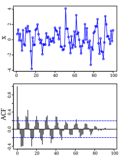
Autocorrelation, sometimes known as serial correlation in the discrete time case, is the correlation of a signal with a delayed copy of itself as a function of delay. Informally, it is the similarity between observations as a function of the time lag between them. The analysis of autocorrelation is a mathematical tool for finding repeating patterns, such as the presence of a periodic signal obscured by noise, or identifying the missing fundamental frequency in a signal implied by its harmonic frequencies. It is often used in signal processing for analyzing functions or series of values, such as time domain signals.

In mathematics, a continuous function is a function such that a continuous variation of the argument induces a continuous variation of the value of the function. This means that there are no abrupt changes in value, known as discontinuities. More precisely, a function is continuous if arbitrarily small changes in its value can be assured by restricting to sufficiently small changes of its argument. A discontinuous function is a function that is not continuous. Up until the 19th century, mathematicians largely relied on intuitive notions of continuity, and considered only continuous functions. The epsilon–delta definition of a limit was introduced to formalize the definition of continuity.

Control theory deals with the control of dynamical systems in engineered processes and machines. The objective is to develop a model or algorithm governing the application of system inputs to drive the system to a desired state, while minimizing any delay, overshoot, or steady-state error and ensuring a level of control stability; often with the aim to achieve a degree of optimality.

In mathematics, convolution is a mathematical operation on two functions that produces a third function that expresses how the shape of one is modified by the other. The term convolution refers to both the result function and to the process of computing it. It is defined as the integral of the product of the two functions after one is reversed and shifted. The integral is evaluated for all values of shift, producing the convolution function.

A phase-locked loop or phase lock loop (PLL) is a control system that generates an output signal whose phase is related to the phase of an input signal. There are several different types; the simplest is an electronic circuit consisting of a variable frequency oscillator and a phase detector in a feedback loop. The oscillator's frequency and phase are controlled proportionally by an applied voltage, hence the term voltage-controlled oscillator (VCO). The oscillator generates a periodic signal of a specific frequency, and the phase detector compares the phase of that signal with the phase of the input periodic signal, to adjust the oscillator to keep the phases matched.

A proportional–integral–derivative controller is a control loop mechanism employing feedback that is widely used in industrial control systems and a variety of other applications requiring continuously modulated control. A PID controller continuously calculates an error value $as the difference between a desired setpoint (SP) and a measured process variable (PV) and applies a correction based on proportional, integral, and derivative terms, hence the name.$

Shear stress, often denoted by $τ$ , is the component of stress coplanar with a material cross section. It arises from the shear force, the component of force vector parallel to the material cross section. Normal stress, on the other hand, arises from the force vector component perpendicular to the material cross section on which it acts.

The step response of a system in a given initial state consists of the time evolution of its outputs when its control inputs are Heaviside step functions. In electronic engineering and control theory, step response is the time behaviour of the outputs of a general system when its inputs change from zero to one in a very short time. The concept can be extended to the abstract mathematical notion of a dynamical system using an evolution parameter.

In mathematics and in signal processing, the Hilbert transform is a specific linear operator that takes a function, $u (t)$ of a real variable and produces another function of a real variable $H(u)(t)$ . This linear operator is given by convolution with the function $. The Hilbert transform has a particularly simple representation in the frequency domain: It imparts a phase shift of \pm90° to every frequency component of a function, the sign of the shift depending on the sign of the frequency. The Hilbert transform is important in signal processing, where it is a component of the analytic representation of a real-valued signal u (t) . The Hilbert transform was first introduced by David Hilbert in this setting, to solve a special case of the Riemann-Hilbert problem for analytic functions.$

In electronics, when describing a voltage or current step function, rise time is the time taken by a signal to change from a specified low value to a specified high value. These values may be expressed as ratios or, equivalently, as percentages with respect to a given reference value. In analog electronics and digital electronics, these percentages are commonly the 10% and 90% of the output step height: however, other values are commonly used. For applications in control theory, according to Levine, rise time is defined as "the time required for the response to rise from $x%$ to $y%$ of its final value", with 0% to 100% rise time common for underdamped second order systems, 5% to 95% for critically damped and 10% to 90% for overdamped ones. According to Orwiler, the term "rise time" applies to either positive or negative step response, even if a displayed negative excursion is popularly termed fall time.

In system analysis, among other fields of study, a linear time-invariant system is a system that produces an output signal from any input signal subject to the constraints of linearity and time-invariance; these terms are briefly defined below. These properties apply to many important physical systems, in which case the response y(t) of the system to an arbitrary input x(t) can be found directly using convolution: y(t) = x(t) ∗ h(t) where h(t) is called the system's impulse response and ∗ represents convolution. What's more, there are systematic methods for solving any such system, whereas systems not meeting both properties are generally more difficult to solve analytically. A good example of an LTI system is any electrical circuit consisting of resistors, capacitors, inductors and linear amplifiers.

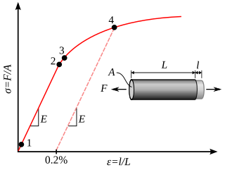
In materials science and engineering, the yield point is the point on a stress-strain curve that indicates the limit of elastic behavior and the beginning of plastic behavior. Below the yield point, a material will deform elastically and will return to its original shape when the applied stress is removed. Once the yield point is passed, some fraction of the deformation will be permanent and non-reversible and is known as plastic deformation.

The Ziegler–Nichols tuning method is a heuristic method of tuning a PID controller. It was developed by John G. Ziegler and Nathaniel B. Nichols. It is performed by setting the I (integral) and D (derivative) gains to zero. The "P" (proportional) gain, $is then increased until it reaches the ultimate gain, at which the output of the control loop has stable and consistent oscillations. and the oscillation period are then used to set the P, I, and D gains depending on the type of controller used and behaviour desired:$

Vector control, also called field-oriented control (FOC), is a variable-frequency drive (VFD) control method in which the stator currents of a three-phase AC or brushless DC electric motor are identified as two orthogonal components that can be visualized with a vector. One component defines the magnetic flux of the motor, the other the torque. The control system of the drive calculates the corresponding current component references from the flux and torque references given by the drive's speed control. Typically proportional-integral (PI) controllers are used to keep the measured current components at their reference values. The pulse-width modulation of the variable-frequency drive defines the transistor switching according to the stator voltage references that are the output of the PI current controllers.

In physics and engineering, the time constant, usually denoted by the Greek letter $τ$ (tau), is the parameter characterizing the response to a step input of a first-order, linear time-invariant (LTI) system. The time constant is the main characteristic unit of a first-order LTI system.

Laser linewidth is the spectral linewidth of a laser beam.

In the mathematical theory of probability, the drift-plus-penalty method is used for optimization of queueing networks and other stochastic systems.

Classical control theory is a branch of control theory that deals with the behavior of dynamical systems with inputs, and how their behavior is modified by feedback, using the Laplace transform as a basic tool to model such systems.

Data-driven control systems are a broad family of control systems, in which the identification of the process model and/or the design of the controller are based entirely on experimental data collected from the plant.

In mathematics and mathematical biology, the Mackey–Glass equations, named after Michael Mackey and Leon Glass, refer to a family of delay differential equations whose behaviour manages to mimic both healthy and pathological behaviour in certain biological contexts, controlled by the equation's parameters. Originally, they were used to model the variation in the relative quantity of mature cells in the blood. The equations are defined as:

References

1 2 Bequette, B. Wayne (2003). Process Control: Modeling, Design, and Simulation. Upper Saddle River, New Jersey: Prentice Hall PTR. pp. 165–168. ISBN 978-0-13-353640-9.

External links

Proportional control compared to on–off or bang–bang control

This page is based on this Wikipedia article
Text is available under the CC BY-SA 4.0 license; additional terms may apply.
Images, videos and audio are available under their respective licenses.

[:0-1] 1 2 Bequette, B. Wayne (2003). Process Control: Modeling, Design, and Simulation. Upper Saddle River, New Jersey: Prentice Hall PTR. pp. 165–168. ISBN 978-0-13-353640-9.

[1]