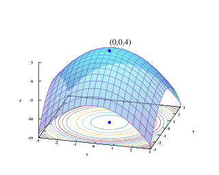
Quadratic programming (QP) is the process of solving certain mathematical optimization problems involving quadratic functions. Specifically, one seeks to optimize a multivariate quadratic function subject to linear constraints on the variables. Quadratic programming is a type of nonlinear programming.

Linear programming (LP), also called linear optimization, is a method to achieve the best outcome in a mathematical model whose requirements and objective are represented by linear relationships. Linear programming is a special case of mathematical programming.
Mathematical optimization or mathematical programming is the selection of a best element, with regard to some criteria, from some set of available alternatives. It is generally divided into two subfields: discrete optimization and continuous optimization. Optimization problems arise in all quantitative disciplines from computer science and engineering to operations research and economics, and the development of solution methods has been of interest in mathematics for centuries.
In mathematical optimization, Dantzig's simplex algorithm is a popular algorithm for linear programming.

Optimal control theory is a branch of control theory that deals with finding a control for a dynamical system over a period of time such that an objective function is optimized. It has numerous applications in science, engineering and operations research. For example, the dynamical system might be a spacecraft with controls corresponding to rocket thrusters, and the objective might be to reach the Moon with minimum fuel expenditure. Or the dynamical system could be a nation's economy, with the objective to minimize unemployment; the controls in this case could be fiscal and monetary policy. A dynamical system may also be introduced to embed operations research problems within the framework of optimal control theory.
An integer programming problem is a mathematical optimization or feasibility program in which some or all of the variables are restricted to be integers. In many settings the term refers to integer linear programming (ILP), in which the objective function and the constraints are linear.
Multi-disciplinary design optimization (MDO) is a field of engineering that uses optimization methods to solve design problems incorporating a number of disciplines. It is also known as multidisciplinary system design optimization (MSDO), and multidisciplinary design analysis and optimization (MDAO).
In mathematics, nonlinear programming (NLP) is the process of solving an optimization problem where some of the constraints are not linear equalities or the objective function is not a linear function. An optimization problem is one of calculation of the extrema of an objective function over a set of unknown real variables and conditional to the satisfaction of a system of equalities and inequalities, collectively termed constraints. It is the sub-field of mathematical optimization that deals with problems that are not linear.
Column generation or delayed column generation is an efficient algorithm for solving large linear programs.
Convex optimization is a subfield of mathematical optimization that studies the problem of minimizing convex functions over convex sets. Many classes of convex optimization problems admit polynomial-time algorithms, whereas mathematical optimization is in general NP-hard.
In mathematical optimization, the Karush–Kuhn–Tucker (KKT) conditions, also known as the Kuhn–Tucker conditions, are first derivative tests for a solution in nonlinear programming to be optimal, provided that some regularity conditions are satisfied.
In mathematical optimization theory, duality or the duality principle is the principle that optimization problems may be viewed from either of two perspectives, the primal problem or the dual problem. If the primal is a minimization problem then the dual is a maximization problem. Any feasible solution to the primal (minimization) problem is at least as large as any feasible solution to the dual (maximization) problem. Therefore, the solution to the primal is an upper bound to the solution of the dual, and the solution of the dual is a lower bound to the solution of the primal. This fact is called weak duality.
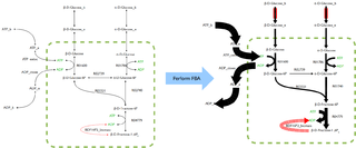
In biochemistry, flux balance analysis (FBA) is a mathematical method for simulating the metabolism of cells or entire unicellular organisms, such as E. coli or yeast, using genome-scale reconstructions of metabolic networks. Genome-scale reconstructions describe all the biochemical reactions in an organism based on its entire genome. These reconstructions model metabolism by focusing on the interactions between metabolites, identifying which metabolites are involved in the various reactions taking place in a cell or organism, and determining the genes that encode the enzymes which catalyze these reactions. In comparison to traditional methods of modeling, FBA is less intensive in terms of the input data required for constructing the model. Simulations performed using FBA are computationally inexpensive and can calculate steady-state metabolic fluxes for large models in a few seconds on modern personal computers. The related method of metabolic pathway analysis seeks to find and list all possible pathways between metabolites.
In mathematical optimization, constrained optimization is the process of optimizing an objective function with respect to some variables in the presence of constraints on those variables. The objective function is either a cost function or energy function, which is to be minimized, or a reward function or utility function, which is to be maximized. Constraints can be either hard constraints, which set conditions for the variables that are required to be satisfied, or soft constraints, which have some variable values that are penalized in the objective function if, and based on the extent that, the conditions on the variables are not satisfied.
Non-linear least squares is the form of least squares analysis used to fit a set of m observations with a model that is non-linear in n unknown parameters (m ≥ n). It is used in some forms of nonlinear regression. The basis of the method is to approximate the model by a linear one and to refine the parameters by successive iterations. There are many similarities to linear least squares, but also some significant differences. In economic theory, the non-linear least squares method is applied in (i) the probit regression, (ii) threshold regression, (iii) smooth regression, (iv) logistic link regression, (v) Box–Cox transformed regressors ().
The dual of a given linear program (LP) is another LP that is derived from the original LP in the following schematic way:
Stochastic control or stochastic optimal control is a sub field of control theory that deals with the existence of uncertainty either in observations or in the noise that drives the evolution of the system. The system designer assumes, in a Bayesian probability-driven fashion, that random noise with known probability distribution affects the evolution and observation of the state variables. Stochastic control aims to design the time path of the controlled variables that performs the desired control task with minimum cost, somehow defined, despite the presence of this noise. The context may be either discrete time or continuous time.
Benders decomposition is a technique in mathematical programming that allows the solution of very large linear programming problems that have a special block structure. This block structure often occurs in applications such as stochastic programming as the uncertainty is usually represented with scenarios. The technique is named after Jacques F. Benders.
In mathematical optimization, linear-fractional programming (LFP) is a generalization of linear programming (LP). Whereas the objective function in a linear program is a linear function, the objective function in a linear-fractional program is a ratio of two linear functions. A linear program can be regarded as a special case of a linear-fractional program in which the denominator is the constant function 1.
In the theory of linear programming, a basic feasible solution (BFS) is a solution with a minimal set of non-zero variables. Geometrically, each BFS corresponds to a vertex of the polyhedron of feasible solutions. If there exists an optimal solution, then there exists an optimal BFS. Hence, to find an optimal solution, it is sufficient to consider the BFS-s. This fact is used by the simplex algorithm, which essentially travels from one BFS to another until an optimal solution is found.


