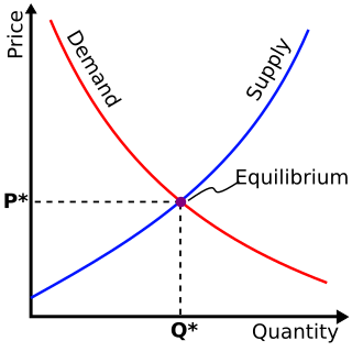
Financial economics is the branch of economics characterized by a "concentration on monetary activities", in which "money of one type or another is likely to appear on both sides of a trade". Its concern is thus the interrelation of financial variables, such as share prices, interest rates and exchange rates, as opposed to those concerning the real economy. It has two main areas of focus: asset pricing and corporate finance; the first being the perspective of providers of capital, i.e. investors, and the second of users of capital. It thus provides the theoretical underpinning for much of finance.

Value at risk (VaR) is a measure of the risk of loss of investment/Capital. It estimates how much a set of investments might lose, given normal market conditions, in a set time period such as a day. VaR is typically used by firms and regulators in the financial industry to gauge the amount of assets needed to cover possible losses.
Market risk is the risk of losses in positions arising from movements in market variables like prices and volatility. There is no unique classification as each classification may refer to different aspects of market risk. Nevertheless, the most commonly used types of market risk are:
Modern portfolio theory (MPT), or mean-variance analysis, is a mathematical framework for assembling a portfolio of assets such that the expected return is maximized for a given level of risk. It is a formalization and extension of diversification in investing, the idea that owning different kinds of financial assets is less risky than owning only one type. Its key insight is that an asset's risk and return should not be assessed by itself, but by how it contributes to a portfolio's overall risk and return. The variance of return is used as a measure of risk, because it is tractable when assets are combined into portfolios. Often, the historical variance and covariance of returns is used as a proxy for the forward-looking versions of these quantities, but other, more sophisticated methods are available.
In finance, arbitrage pricing theory (APT) is a multi-factor model for asset pricing which relates various macro-economic (systematic) risk variables to the pricing of financial assets. Proposed by economist Stephen Ross in 1976, it is widely believed to be an improved alternative to its predecessor, the capital asset pricing model (CAPM). APT is founded upon the law of one price, which suggests that within an equilibrium market, rational investors will implement arbitrage such that the equilibrium price is eventually realised. As such, APT argues that when opportunities for arbitrage are exhausted in a given period, then the expected return of an asset is a linear function of various factors or theoretical market indices, where sensitivities of each factor is represented by a factor-specific beta coefficient or factor loading. Consequently, it provides traders with an indication of ‘true’ asset value and enables exploitation of market discrepancies via arbitrage. The linear factor model structure of the APT is used as the basis for evaluating asset allocation, the performance of managed funds as well as the calculation of cost of capital. Furthermore, the newer APT model is more dynamic being utilised in more theoretical application than the preceding CAPM model. A 1986 article written by Gregory Connor and Robert Korajczyk, utilised the APT framework and applied it to portfolio performance measurement suggesting that the Jensen coefficient is an acceptable measurement of portfolio performance.
In finance, the beta is a statistic that measures the expected increase or decrease of an individual stock price in proportion to movements of the stock market as a whole. Beta can be used to indicate the contribution of an individual asset to the market risk of a portfolio when it is added in small quantity. It refers to an asset's non-diversifiable risk, systematic risk, or market risk. Beta is not a measure of idiosyncratic risk.
Financial risk management is the practice of protecting economic value in a firm by managing exposure to financial risk - principally operational risk, credit risk and market risk, with more specific variants as listed aside. As for risk management more generally, financial risk management requires identifying the sources of risk, measuring these, and crafting plans to mitigate them. See Finance § Risk management for an overview.
Financial risk is any of various types of risk associated with financing, including financial transactions that include company loans in risk of default. Often it is understood to include only downside risk, meaning the potential for financial loss and uncertainty about its extent.
Financial risk modeling is the use of formal mathematical and econometric techniques to measure, monitor and control the market risk, credit risk, and operational risk on a firm's balance sheet, on a bank's accounting ledger of tradeable financial assets, or of a fund manager's portfolio value; see Financial risk management. Risk modeling is one of many subtasks within the broader area of financial modeling.
The following outline is provided as an overview of and topical guide to finance:
The single-index model (SIM) is a simple asset pricing model to measure both the risk and the return of a stock. The model has been developed by William Sharpe in 1963 and is commonly used in the finance industry. Mathematically the SIM is expressed as:
Simply stated, post-modern portfolio theory (PMPT) is an extension of the traditional modern portfolio theory (MPT) of Markowitz and Sharpe. Both theories provide analytical methods for rational investors to use diversification to optimize their investment portfolios. The essential difference between PMPT and MPT is that PMPT emphasizes the return that must be earned on an investment in order to meet future, specified obligations, MPT is concerned only with the absolute return vis-a-vis the risk-free rate.

In finance, volatility is the degree of variation of a trading price series over time, usually measured by the standard deviation of logarithmic returns.
In finance, model risk is the risk of loss resulting from using insufficiently accurate models to make decisions, originally and frequently in the context of valuing financial securities.
Tail risk, sometimes called "fat tail risk," is the financial risk of an asset or portfolio of assets moving more than three standard deviations from its current price, above the risk of a normal distribution. Tail risks include low-probability events arising at both ends of a normal distribution curve, also known as tail events. However, as investors are generally more concerned with unexpected losses rather than gains, a debate about tail risk is focused on the left tail. Prudent asset managers are typically cautious with the tail involving losses which could damage or ruin portfolios, and not the beneficial tail of outsized gains.
In investment banking, PnL explained is an income statement with commentary that attributes or explains the daily fluctuation in the value of a portfolio of trades to the root causes of the changes.
In finance, a stress test is an analysis or simulation designed to determine the ability of a given financial instrument or financial institution to deal with an economic crisis. Instead of doing financial projection on a "best estimate" basis, a company or its regulators may do stress testing where they look at how robust a financial instrument is in certain crashes, a form of scenario analysis. They may test the instrument under, for example, the following stresses:

Portfolio optimization is the process of selecting an optimal portfolio, out of a set of considered portfolios, according to some objective. The objective typically maximizes factors such as expected return, and minimizes costs like financial risk, resulting in a multi-objective optimization problem. Factors being considered may range from tangible to intangible.
Mathematical finance, also known as quantitative finance and financial mathematics, is a field of applied mathematics, concerned with mathematical modeling in the financial field.
In finance, the Markowitz model ─ put forward by Harry Markowitz in 1952 ─ is a portfolio optimization model; it assists in the selection of the most efficient portfolio by analyzing various possible portfolios of the given securities. Here, by choosing securities that do not 'move' exactly together, the HM model shows investors how to reduce their risk. The HM model is also called mean-variance model due to the fact that it is based on expected returns (mean) and the standard deviation (variance) of the various portfolios. It is foundational to Modern portfolio theory.


