Algorithm
Main loop
On each iteration we shift in  digits of the radicand, so we have
  and we produce one digit of the root, so we have
  . The first invariant implies that
  . We want to choose
  so that the invariants described above hold. It turns out that there is always exactly one such choice, as will be proved below.
Proof of existence and uniqueness of By definition of a digit,  , and by definition of a block of digits,
The first invariant says that:

or

So, pick the largest integer such that

Such a always exists, since and if  then
then  , but since
  , this is always true for . Thus, there will always be a that satisfies the first invariant
Now consider the second invariant. It says:

or

Now, if is not the largest admissible for the first invariant as described above, then  is also admissible, and we have

This violates the second invariant, so to satisfy both invariants we must pick the largest allowed by the first invariant. Thus we have proven the existence and uniqueness of .
To summarize, on each iteration:
- Let
 be the next aligned block of digits from the radicand
 - Let
- Let be the largest such that

- Let
- Let
Now, note that  , so the condition
is equivalent to

and

is equivalent to

Thus, we do not actually need  , and since
  and
and  ,
,  or
or  , or
, or  , so by using
  instead of we save time and space by a factor of 1/. Also, the
  we subtract in the new test cancels the one in
  , so now the highest power of
  we have to evaluate is
  rather than
  .
.
Summary
- Initialize and to 0.
- Repeat until desired precision is obtained:
- Let be the next aligned block of digits from the radicand.
- Let be the largest such that

- Let .
- Let
- Assign
 and
and 
- is the largest integer such that
 , and
, and  , where
  is the number of digits of the radicand after the decimal point that have been consumed (a negative number if the algorithm has not reached the decimal point yet).
On each iteration, the most time-consuming task is to select . We know that there are  possible values, so we can find using
  comparisons. Each comparison will require evaluating
  . In the kth iteration, has digits, and the polynomial can be evaluated with
  multiplications of up to
  digits and
  additions of up to digits, once we know the powers of and up through
  for and for . has a restricted range, so we can get the powers of in constant time. We can get the powers of with multiplications of up to digits. Assuming -digit multiplication takes time
  and addition takes time
  , we take time
  for each comparison, or time
  to pick . The remainder of the algorithm is addition and subtraction that takes time
  , so each iteration takes . For all digits, we need time
  .
.
The only internal storage needed is , which is digits on the kth iteration. That this algorithm does not have bounded memory usage puts an upper bound on the number of digits which can be computed mentally, unlike the more elementary algorithms of arithmetic. Unfortunately, any bounded memory state machine with periodic inputs can only produce periodic outputs, so there are no such algorithms which can compute irrational numbers from rational ones, and thus no bounded memory root extraction algorithms.
Note that increasing the base increases the time needed to pick by a factor of  , but decreases the number of digits needed to achieve a given precision by the same factor, and since the algorithm is cubic time in the number of digits, increasing the base gives an overall speedup of
  . When the base is larger than the radicand, the algorithm degenerates to binary search, so it follows that this algorithm is not useful for computing roots with a computer, as it is always outperformed by much simpler binary search, and has the same memory complexity.
In arithmetic, long division is a standard division algorithm suitable for dividing multi-digit Hindu-Arabic numerals that is simple enough to perform by hand. It breaks down a division problem into a series of easier steps.

Lagrange's four-square theorem, also known as Bachet's conjecture, states that every natural number can be represented as a sum of four non-negative integer squares. That is, the squares form an additive basis of order four.
Multi-index notation is a mathematical notation that simplifies formulas used in multivariable calculus, partial differential equations and the theory of distributions, by generalising the concept of an integer index to an ordered tuple of indices.

In geometry, Euler's rotation theorem states that, in three-dimensional space, any displacement of a rigid body such that a point on the rigid body remains fixed, is equivalent to a single rotation about some axis that runs through the fixed point. It also means that the composition of two rotations is also a rotation. Therefore the set of rotations has a group structure, known as a rotation group.
In mathematics, the Smith normal form is a normal form that can be defined for any matrix with entries in a principal ideal domain (PID). The Smith normal form of a matrix is diagonal, and can be obtained from the original matrix by multiplying on the left and right by invertible square matrices. In particular, the integers are a PID, so one can always calculate the Smith normal form of an integer matrix. The Smith normal form is very useful for working with finitely generated modules over a PID, and in particular for deducing the structure of a quotient of a free module. It is named after the Irish mathematician Henry John Stephen Smith.
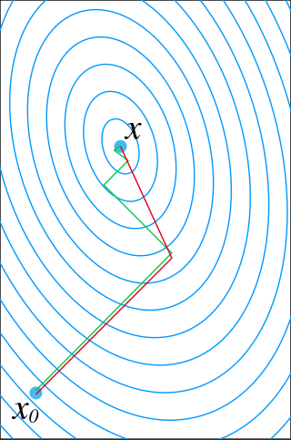
In mathematics, the conjugate gradient method is an algorithm for the numerical solution of particular systems of linear equations, namely those whose matrix is positive-semidefinite. The conjugate gradient method is often implemented as an iterative algorithm, applicable to sparse systems that are too large to be handled by a direct implementation or other direct methods such as the Cholesky decomposition. Large sparse systems often arise when numerically solving partial differential equations or optimization problems.
In the field of mathematics, norms are defined for elements within a vector space. Specifically, when the vector space comprises matrices, such norms are referred to as matrix norms. Matrix norms differ from vector norms in that they must also interact with matrix multiplication.
Exponential smoothing or exponential moving average (EMA) is a rule of thumb technique for smoothing time series data using the exponential window function. Whereas in the simple moving average the past observations are weighted equally, exponential functions are used to assign exponentially decreasing weights over time. It is an easily learned and easily applied procedure for making some determination based on prior assumptions by the user, such as seasonality. Exponential smoothing is often used for analysis of time-series data.
In numerical optimization, the Broyden–Fletcher–Goldfarb–Shanno (BFGS) algorithm is an iterative method for solving unconstrained nonlinear optimization problems. Like the related Davidon–Fletcher–Powell method, BFGS determines the descent direction by preconditioning the gradient with curvature information. It does so by gradually improving an approximation to the Hessian matrix of the loss function, obtained only from gradient evaluations via a generalized secant method.
In mathematics, the resultant of two polynomials is a polynomial expression of their coefficients that is equal to zero if and only if the polynomials have a common root, or, equivalently, a common factor. In some older texts, the resultant is also called the eliminant.
In mathematics, a real or complex-valued function f on d-dimensional Euclidean space satisfies a Hölder condition, or is Hölder continuous, when there are real constants C ≥ 0, > 0, such that
In computational complexity theory, PostBQP is a complexity class consisting of all of the computational problems solvable in polynomial time on a quantum Turing machine with postselection and bounded error.
In numerical optimization, the nonlinear conjugate gradient method generalizes the conjugate gradient method to nonlinear optimization. For a quadratic function
A ratio distribution is a probability distribution constructed as the distribution of the ratio of random variables having two other known distributions. Given two random variables X and Y, the distribution of the random variable Z that is formed as the ratio Z = X/Y is a ratio distribution.
In statistics, the generalized Dirichlet distribution (GD) is a generalization of the Dirichlet distribution with a more general covariance structure and almost twice the number of parameters. Random vectors with a GD distribution are completely neutral.
A self-concordant function is a function satisfying a certain differential inequality, which makes it particularly easy for optimization using Newton's method A self-concordant barrier is a particular self-concordant function, that is also a barrier function for a particular convex set. Self-concordant barriers are important ingredients in interior point methods for optimization.
The factorization of a linear partial differential operator (LPDO) is an important issue in the theory of integrability, due to the Laplace-Darboux transformations, which allow construction of integrable LPDEs. Laplace solved the factorization problem for a bivariate hyperbolic operator of the second order, constructing two Laplace invariants. Each Laplace invariant is an explicit polynomial condition of factorization; coefficients of this polynomial are explicit functions of the coefficients of the initial LPDO. The polynomial conditions of factorization are called invariants because they have the same form for equivalent operators.
In coding theory, list decoding is an alternative to unique decoding of error-correcting codes in the presence of many errors. If a code has relative distance , then it is possible in principle to recover an encoded message when up to fraction of the codeword symbols are corrupted. But when error rate is greater than , this will not in general be possible. List decoding overcomes that issue by allowing the decoder to output a short list of messages that might have been encoded. List decoding can correct more than fraction of errors.

In computer science, a suffix automaton is an efficient data structure for representing the substring index of a given string which allows the storage, processing, and retrieval of compressed information about all its substrings. The suffix automaton of a string is the smallest directed acyclic graph with a dedicated initial vertex and a set of "final" vertices, such that paths from the initial vertex to final vertices represent the suffixes of the string.
In computational learning theory, Occam learning is a model of algorithmic learning where the objective of the learner is to output a succinct representation of received training data. This is closely related to probably approximately correct (PAC) learning, where the learner is evaluated on its predictive power of a test set.


