
Bessel functions, first defined by the mathematician Daniel Bernoulli and then generalized by Friedrich Bessel, are canonical solutions y(x) of Bessel's differential equation for an arbitrary complex number , which represents the order of the Bessel function. Although and produce the same differential equation, it is conventional to define different Bessel functions for these two values in such a way that the Bessel functions are mostly smooth functions of .
In computational mathematics, an iterative method is a mathematical procedure that uses an initial value to generate a sequence of improving approximate solutions for a class of problems, in which the i-th approximation is derived from the previous ones.
A finite difference is a mathematical expression of the form f (x + b) − f (x + a). If a finite difference is divided by b − a, one gets a difference quotient. The approximation of derivatives by finite differences plays a central role in finite difference methods for the numerical solution of differential equations, especially boundary value problems.

In mathematics, the Lambert W function, also called the omega function or product logarithm, is a multivalued function, namely the branches of the converse relation of the function f(w) = wew, where w is any complex number and ew is the exponential function. The function is named after Johann Lambert, who considered a related problem in 1758. Building on Lambert's work, Leonhard Euler described the W function per se in 1783.

In analysis, numerical integration comprises a broad family of algorithms for calculating the numerical value of a definite integral. The term numerical quadrature is more or less a synonym for "numerical integration", especially as applied to one-dimensional integrals. Some authors refer to numerical integration over more than one dimension as cubature; others take "quadrature" to include higher-dimensional integration.

Numerical methods for ordinary differential equations are methods used to find numerical approximations to the solutions of ordinary differential equations (ODEs). Their use is also known as "numerical integration", although this term can also refer to the computation of integrals.
Pseudo-spectral methods, also known as discrete variable representation (DVR) methods, are a class of numerical methods used in applied mathematics and scientific computing for the solution of partial differential equations. They are closely related to spectral methods, but complement the basis by an additional pseudo-spectral basis, which allows representation of functions on a quadrature grid. This simplifies the evaluation of certain operators, and can considerably speed up the calculation when using fast algorithms such as the fast Fourier transform.
In mathematical analysis, asymptotic analysis, also known as asymptotics, is a method of describing limiting behavior.
In mathematical analysis, particularly numerical analysis, the rate of convergence and order of convergence of a sequence that converges to a limit are any of several characterizations of how quickly that sequence approaches its limit. These are broadly divided into rates and orders of convergence that describe how quickly a sequence further approaches its limit once it is already close to it, called asymptotic rates and orders of convergence, and those that describe how quickly sequences approach their limits from starting points that are not necessarily close to their limits, called non-asymptotic rates and orders of convergence.
In mathematics, the Helmholtz equation is the eigenvalue problem for the Laplace operator. It corresponds to the elliptic partial differential equation: where ∇2 is the Laplace operator, k2 is the eigenvalue, and f is the (eigen)function. When the equation is applied to waves, k is known as the wave number. The Helmholtz equation has a variety of applications in physics and other sciences, including the wave equation, the diffusion equation, and the Schrödinger equation for a free particle.
A stochastic differential equation (SDE) is a differential equation in which one or more of the terms is a stochastic process, resulting in a solution which is also a stochastic process. SDEs have many applications throughout pure mathematics and are used to model various behaviours of stochastic models such as stock prices, random growth models or physical systems that are subjected to thermal fluctuations.

In mathematics, a series expansion is a technique that expresses a function as an infinite sum, or series, of simpler functions. It is a method for calculating a function that cannot be expressed by just elementary operators.
In mathematics, a fundamental solution for a linear partial differential operator L is a formulation in the language of distribution theory of the older idea of a Green's function.
In mathematics, a stiff equation is a differential equation for which certain numerical methods for solving the equation are numerically unstable, unless the step size is taken to be extremely small. It has proven difficult to formulate a precise definition of stiffness, but the main idea is that the equation includes some terms that can lead to rapid variation in the solution.
In mathematics a radial basis function (RBF) is a real-valued function whose value depends only on the distance between the input and some fixed point, either the origin, so that , or some other fixed point , called a center, so that . Any function that satisfies the property is a radial function. The distance is usually Euclidean distance, although other metrics are sometimes used. They are often used as a collection which forms a basis for some function space of interest, hence the name.

In mathematics, a Padé approximant is the "best" approximation of a function near a specific point by a rational function of given order. Under this technique, the approximant's power series agrees with the power series of the function it is approximating. The technique was developed around 1890 by Henri Padé, but goes back to Georg Frobenius, who introduced the idea and investigated the features of rational approximations of power series.
In numerical analysis, finite-difference methods (FDM) are a class of numerical techniques for solving differential equations by approximating derivatives with finite differences. Both the spatial domain and time domain are discretized, or broken into a finite number of intervals, and the values of the solution at the end points of the intervals are approximated by solving algebraic equations containing finite differences and values from nearby points.
In applied mathematics, polyharmonic splines are used for function approximation and data interpolation. They are very useful for interpolating and fitting scattered data in many dimensions. Special cases include thin plate splines and natural cubic splines in one dimension.
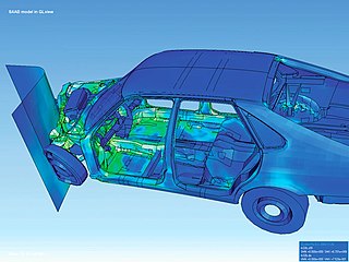
The finite element method (FEM) is a popular method for numerically solving differential equations arising in engineering and mathematical modeling. Typical problem areas of interest include the traditional fields of structural analysis, heat transfer, fluid flow, mass transport, and electromagnetic potential.
The Kansa method is a computer method used to solve partial differential equations. Its main advantage is it is very easy to understand and program on a computer. It is much less complicated than the finite element method. Another advantage is it works well on multi variable problems. The finite element method is complicated when working with more than 3 space variables and time.


