The method of least squares is a standard approach in regression analysis to approximate the solution of overdetermined systems by minimizing the sum of the squares of the residuals made in the results of each individual equation.

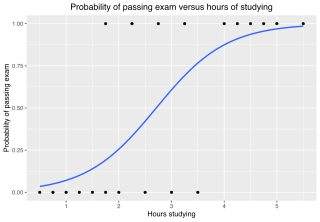
In statistics, the logistic model is a statistical model that models the probability of an event taking place by having the log-odds for the event be a linear combination of one or more independent variables. In regression analysis, logistic regression is estimating the parameters of a logistic model. Formally, in binary logistic regression there is a single binary dependent variable, coded by an indicator variable, where the two values are labeled "0" and "1", while the independent variables can each be a binary variable or a continuous variable. The corresponding probability of the value labeled "1" can vary between 0 and 1, hence the labeling; the function that converts log-odds to probability is the logistic function, hence the name. The unit of measurement for the log-odds scale is called a logit, from logistic unit, hence the alternative names. See § Background and § Definition for formal mathematics, and § Example for a worked example.
Simultaneous equations models are a type of statistical model in which the dependent variables are functions of other dependent variables, rather than just independent variables. This means some of the explanatory variables are jointly determined with the dependent variable, which in economics usually is the consequence of some underlying equilibrium mechanism. Take the typical supply and demand model: whilst typically one would determine the quantity supplied and demanded to be a function of the price set by the market, it is also possible for the reverse to be true, where producers observe the quantity that consumers demand and then set the price.
In statistical inference, specifically predictive inference, a prediction interval is an estimate of an interval in which a future observation will fall, with a certain probability, given what has already been observed. Prediction intervals are often used in regression analysis.
Empirical Bayes methods are procedures for statistical inference in which the prior probability distribution is estimated from the data. This approach stands in contrast to standard Bayesian methods, for which the prior distribution is fixed before any data are observed. Despite this difference in perspective, empirical Bayes may be viewed as an approximation to a fully Bayesian treatment of a hierarchical model wherein the parameters at the highest level of the hierarchy are set to their most likely values, instead of being integrated out. Empirical Bayes, also known as maximum marginal likelihood, represents a convenient approach for setting hyperparameters, but has been mostly supplanted by fully Bayesian hierarchical analyses since the 2000s with the increasing availability of well-performing computation techniques. It is still commonly used, however, for variational methods in Deep Learning, such as variational autoencoders, where latent variable spaces are high-dimensional.
In statistics, a generalized linear model (GLM) is a flexible generalization of ordinary linear regression. The GLM generalizes linear regression by allowing the linear model to be related to the response variable via a link function and by allowing the magnitude of the variance of each measurement to be a function of its predicted value.

In statistics, the coefficient of determination, denoted R2 or r2 and pronounced "R squared", is the proportion of the variation in the dependent variable that is predictable from the independent variable(s).
In statistics, a probit model is a type of regression where the dependent variable can take only two values, for example married or not married. The word is a portmanteau, coming from probability + unit. The purpose of the model is to estimate the probability that an observation with particular characteristics will fall into a specific one of the categories; moreover, classifying observations based on their predicted probabilities is a type of binary classification model.
In statistics, a generalized additive model (GAM) is a generalized linear model in which the linear response variable depends linearly on unknown smooth functions of some predictor variables, and interest focuses on inference about these smooth functions.
Multilevel models are statistical models of parameters that vary at more than one level. An example could be a model of student performance that contains measures for individual students as well as measures for classrooms within which the students are grouped. These models can be seen as generalizations of linear models, although they can also extend to non-linear models. These models became much more popular after sufficient computing power and software became available.
In statistics, binomial regression is a regression analysis technique in which the response has a binomial distribution: it is the number of successes in a series of independent Bernoulli trials, where each trial has probability of success . In binomial regression, the probability of a success is related to explanatory variables: the corresponding concept in ordinary regression is to relate the mean value of the unobserved response to explanatory variables.

In probability theory and statistics, the beta-binomial distribution is a family of discrete probability distributions on a finite support of non-negative integers arising when the probability of success in each of a fixed or known number of Bernoulli trials is either unknown or random. The beta-binomial distribution is the binomial distribution in which the probability of success at each of n trials is not fixed but randomly drawn from a beta distribution. It is frequently used in Bayesian statistics, empirical Bayes methods and classical statistics to capture overdispersion in binomial type distributed data.
Bayesian linear regression is a type of conditional modeling in which the mean of one variable is described by a linear combination of other variables, with the goal of obtaining the posterior probability of the regression coefficients and ultimately allowing the out-of-sample prediction of the regressandconditional on observed values of the regressors. The simplest and most widely used version of this model is the normal linear model, in which given is distributed Gaussian. In this model, and under a particular choice of prior probabilities for the parameters—so-called conjugate priors—the posterior can be found analytically. With more arbitrarily chosen priors, the posteriors generally have to be approximated.
In statistics, regression validation is the process of deciding whether the numerical results quantifying hypothesized relationships between variables, obtained from regression analysis, are acceptable as descriptions of the data. The validation process can involve analyzing the goodness of fit of the regression, analyzing whether the regression residuals are random, and checking whether the model's predictive performance deteriorates substantially when applied to data that were not used in model estimation.
The Heckman correction is a statistical technique to correct bias from non-randomly selected samples or otherwise incidentally truncated dependent variables, a pervasive issue in quantitative social sciences when using observational data. Conceptually, this is achieved by explicitly modelling the individual sampling probability of each observation together with the conditional expectation of the dependent variable. The resulting likelihood function is mathematically similar to the tobit model for censored dependent variables, a connection first drawn by James Heckman in 1974. Heckman also developed a two-step control function approach to estimate this model, which avoids the computational burden of having to estimate both equations jointly, albeit at the cost of inefficiency. Heckman received the Nobel Memorial Prize in Economic Sciences in 2000 for his work in this field.
In statistics and machine learning, lasso is a regression analysis method that performs both variable selection and regularization in order to enhance the prediction accuracy and interpretability of the resulting statistical model. It was originally introduced in geophysics, and later by Robert Tibshirani, who coined the term.
In statistics, the g-prior is an objective prior for the regression coefficients of a multiple regression. It was introduced by Arnold Zellner. It is a key tool in Bayes and empirical Bayes variable selection.
In statistics, linear regression is a linear approach for modelling the relationship between a scalar response and one or more explanatory variables. The case of one explanatory variable is called simple linear regression; for more than one, the process is called multiple linear regression. This term is distinct from multivariate linear regression, where multiple correlated dependent variables are predicted, rather than a single scalar variable.
Bayesian structural time series (BSTS) model is a statistical technique used for feature selection, time series forecasting, nowcasting, inferring causal impact and other applications. The model is designed to work with time series data.


