
In vector calculus, divergence is a vector operator that operates on a vector field, producing a scalar field giving the quantity of the vector field's source at each point. More technically, the divergence represents the volume density of the outward flux of a vector field from an infinitesimal volume around a given point.
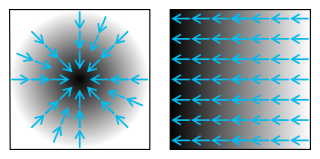
In vector calculus, the gradient of a scalar-valued differentiable function f of several variables is the vector field whose value at a point is the "direction and rate of fastest increase". If the gradient of a function is non-zero at a point p, the direction of the gradient is the direction in which the function increases most quickly from p, and the magnitude of the gradient is the rate of increase in that direction, the greatest absolute directional derivative. Further, a point where the gradient is the zero vector is known as a stationary point. The gradient thus plays a fundamental role in optimization theory, where it is used to maximize a function by gradient ascent. In coordinate-free terms, the gradient of a function may be defined by:

In physics, the Lorentz transformations are a six-parameter family of linear transformations from a coordinate frame in spacetime to another frame that moves at a constant velocity relative to the former. The respective inverse transformation is then parameterized by the negative of this velocity. The transformations are named after the Dutch physicist Hendrik Lorentz.

In mathematics, a tensor is an algebraic object that describes a multilinear relationship between sets of algebraic objects related to a vector space. Tensors may map between different objects such as vectors, scalars, and even other tensors. There are many types of tensors, including scalars and vectors, dual vectors, multilinear maps between vector spaces, and even some operations such as the dot product. Tensors are defined independent of any basis, although they are often referred to by their components in a basis related to a particular coordinate system.
In mathematics, especially the usage of linear algebra in mathematical physics, Einstein notation is a notational convention that implies summation over a set of indexed terms in a formula, thus achieving brevity. As part of mathematics it is a notational subset of Ricci calculus; however, it is often used in physics applications that do not distinguish between tangent and cotangent spaces. It was introduced to physics by Albert Einstein in 1916.
In the mathematical field of differential geometry, a metric tensor is an additional structure on a manifold M that allows defining distances and angles, just as the inner product on a Euclidean space allows defining distances and angles there. More precisely, a metric tensor at a point p of M is a bilinear form defined on the tangent space at p, and a metric tensor on M consists of a metric tensor at each point p of M that varies smoothly with p.
In multilinear algebra, a tensor contraction is an operation on a tensor that arises from the natural pairing of a finite-dimensional vector space and its dual. In components, it is expressed as a sum of products of scalar components of the tensor(s) caused by applying the summation convention to a pair of dummy indices that are bound to each other in an expression. The contraction of a single mixed tensor occurs when a pair of literal indices of the tensor are set equal to each other and summed over. In Einstein notation this summation is built into the notation. The result is another tensor with order reduced by 2.

In physics, especially in multilinear algebra and tensor analysis, covariance and contravariance describe how the quantitative description of certain geometric or physical entities changes with a change of basis. In modern mathematical notation, the role is sometimes swapped.
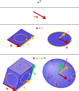
In mathematics, the exterior algebra, or Grassmann algebra, named after Hermann Grassmann, is an algebra that uses the exterior product or wedge product as its multiplication. In mathematics, the exterior product or wedge product of vectors is an algebraic construction used in geometry to study areas, volumes, and their higher-dimensional analogues. The exterior product of two vectors and denoted by is called a bivector and lives in a space called the exterior square, a vector space that is distinct from the original space of vectors. The magnitude of can be interpreted as the area of the parallelogram with sides and which in three dimensions can also be computed using the cross product of the two vectors. More generally, all parallel plane surfaces with the same orientation and area have the same bivector as a measure of their oriented area. Like the cross product, the exterior product is anticommutative, meaning that for all vectors and but, unlike the cross product, the exterior product is associative.
In mathematics and physics, a tensor field assigns a tensor to each point of a mathematical space. Tensor fields are used in differential geometry, algebraic geometry, general relativity, in the analysis of stress and strain in materials, and in numerous applications in the physical sciences. As a tensor is a generalization of a scalar and a vector, a tensor field is a generalization of a scalar field or vector field that assigns, respectively, a scalar or vector to each point of space. If a tensor A is defined on a vector fields set X(M) over a module M, we call A a tensor field on M.
In mathematics, and especially differential geometry and gauge theory, a connection on a fiber bundle is a device that defines a notion of parallel transport on the bundle; that is, a way to "connect" or identify fibers over nearby points. The most common case is that of a linear connection on a vector bundle, for which the notion of parallel transport must be linear. A linear connection is equivalently specified by a covariant derivative, an operator that differentiates sections of the bundle along tangent directions in the base manifold, in such a way that parallel sections have derivative zero. Linear connections generalize, to arbitrary vector bundles, the Levi-Civita connection on the tangent bundle of a pseudo-Riemannian manifold, which gives a standard way to differentiate vector fields. Nonlinear connections generalize this concept to bundles whose fibers are not necessarily linear.
In mathematics, the covariant derivative is a way of specifying a derivative along tangent vectors of a manifold. Alternatively, the covariant derivative is a way of introducing and working with a connection on a manifold by means of a differential operator, to be contrasted with the approach given by a principal connection on the frame bundle – see affine connection. In the special case of a manifold isometrically embedded into a higher-dimensional Euclidean space, the covariant derivative can be viewed as the orthogonal projection of the Euclidean directional derivative onto the manifold's tangent space. In this case the Euclidean derivative is broken into two parts, the extrinsic normal component and the intrinsic covariant derivative component.

In physics, a covariant transformation is a rule that specifies how certain entities, such as vectors or tensors, change under a change of basis. The transformation that describes the new basis vectors as a linear combination of the old basis vectors is defined as a covariant transformation. Conventionally, indices identifying the basis vectors are placed as lower indices and so are all entities that transform in the same way. The inverse of a covariant transformation is a contravariant transformation. Whenever a vector should be invariant under a change of basis, that is to say it should represent the same geometrical or physical object having the same magnitude and direction as before, its components must transform according to the contravariant rule. Conventionally, indices identifying the components of a vector are placed as upper indices and so are all indices of entities that transform in the same way. The sum over pairwise matching indices of a product with the same lower and upper indices are invariant under a transformation.
In mathematics, and specifically differential geometry, a connection form is a manner of organizing the data of a connection using the language of moving frames and differential forms.
In mathematics, the Kronecker product, sometimes denoted by ⊗, is an operation on two matrices of arbitrary size resulting in a block matrix. It is a specialization of the tensor product from vectors to matrices and gives the matrix of the tensor product linear map with respect to a standard choice of basis. The Kronecker product is to be distinguished from the usual matrix multiplication, which is an entirely different operation. The Kronecker product is also sometimes called matrix direct product.
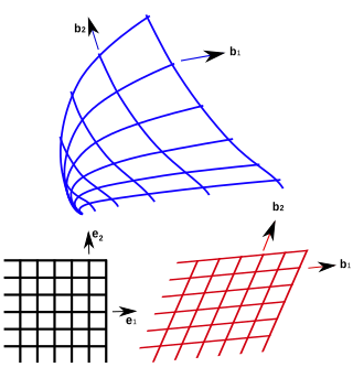
In geometry, curvilinear coordinates are a coordinate system for Euclidean space in which the coordinate lines may be curved. These coordinates may be derived from a set of Cartesian coordinates by using a transformation that is locally invertible at each point. This means that one can convert a point given in a Cartesian coordinate system to its curvilinear coordinates and back. The name curvilinear coordinates, coined by the French mathematician Lamé, derives from the fact that the coordinate surfaces of the curvilinear systems are curved.
In mathematics and physics, the Christoffel symbols are an array of numbers describing a metric connection. The metric connection is a specialization of the affine connection to surfaces or other manifolds endowed with a metric, allowing distances to be measured on that surface. In differential geometry, an affine connection can be defined without reference to a metric, and many additional concepts follow: parallel transport, covariant derivatives, geodesics, etc. also do not require the concept of a metric. However, when a metric is available, these concepts can be directly tied to the "shape" of the manifold itself; that shape is determined by how the tangent space is attached to the cotangent space by the metric tensor. Abstractly, one would say that the manifold has an associated (orthonormal) frame bundle, with each "frame" being a possible choice of a coordinate frame. An invariant metric implies that the structure group of the frame bundle is the orthogonal group O(p, q). As a result, such a manifold is necessarily a (pseudo-)Riemannian manifold. The Christoffel symbols provide a concrete representation of the connection of (pseudo-)Riemannian geometry in terms of coordinates on the manifold. Additional concepts, such as parallel transport, geodesics, etc. can then be expressed in terms of Christoffel symbols.

In geometry and linear algebra, a Cartesian tensor uses an orthonormal basis to represent a tensor in a Euclidean space in the form of components. Converting a tensor's components from one such basis to another is through an orthogonal transformation.
In mathematics—more specifically, in differential geometry—the musical isomorphism is an isomorphism between the tangent bundle and the cotangent bundle of a pseudo-Riemannian manifold induced by its metric tensor. There are similar isomorphisms on symplectic manifolds. The term musical refers to the use of the symbols (flat) and (sharp).
Curvilinear coordinates can be formulated in tensor calculus, with important applications in physics and engineering, particularly for describing transportation of physical quantities and deformation of matter in fluid mechanics and continuum mechanics.


