In mathematics and statistics, the arithmetic mean, arithmetic average, or just the mean or average is the sum of a collection of numbers divided by the count of numbers in the collection. The collection is often a set of results from an experiment, an observational study, or a survey. The term "arithmetic mean" is preferred in some mathematics and statistics contexts because it helps distinguish it from other types of means, such as geometric and harmonic.
A histogram is a visual representation of the distribution of quantitative data. To construct a histogram, the first step is to "bin" the range of values— divide the entire range of values into a series of intervals—and then count how many values fall into each interval. The bins are usually specified as consecutive, non-overlapping intervals of a variable. The bins (intervals) are adjacent and are typically of equal size.

In statistics, stratified sampling is a method of sampling from a population which can be partitioned into subpopulations.
In statistics, an effect size is a value measuring the strength of the relationship between two variables in a population, or a sample-based estimate of that quantity. It can refer to the value of a statistic calculated from a sample of data, the value of one parameter for a hypothetical population, or to the equation that operationalizes how statistics or parameters lead to the effect size value. Examples of effect sizes include the correlation between two variables, the regression coefficient in a regression, the mean difference, or the risk of a particular event happening. Effect sizes are a complement tool for statistical hypothesis testing, and play an important role in power analyses to assess the sample size required for new experiments. Effect size are fundamental in meta-analyses which aim to provide the combined effect size based on data from multiple studies. The cluster of data-analysis methods concerning effect sizes is referred to as estimation statistics.
Student's t-test is a statistical test used to test whether the difference between the response of two groups is statistically significant or not. It is any statistical hypothesis test in which the test statistic follows a Student's t-distribution under the null hypothesis. It is most commonly applied when the test statistic would follow a normal distribution if the value of a scaling term in the test statistic were known. When the scaling term is estimated based on the data, the test statistic—under certain conditions—follows a Student's t distribution. The t-test's most common application is to test whether the means of two populations are significantly different. In many cases, a Z-test will yield very similar results to a t-test because the latter converges to the former as the size of the dataset increases.
Pixels per inch (ppi) and pixels per centimetre are measurements of the pixel density of an electronic image device, such as a computer monitor or television display, or image digitizing device such as a camera or image scanner. Horizontal and vertical density are usually the same, as most devices have square pixels, but differ on devices that have non-square pixels. Pixel density is not the same as resolution — where the former describes the amount of detail on a physical surface or device, the latter describes the amount of pixel information regardless of its scale. Considered in another way, a pixel has no inherent size or unit, but when it is printed, displayed, or scanned, then the pixel has both a physical size (dimension) and a pixel density (ppi).
Sample size determination or estimation is the act of choosing the number of observations or replicates to include in a statistical sample. The sample size is an important feature of any empirical study in which the goal is to make inferences about a population from a sample. In practice, the sample size used in a study is usually determined based on the cost, time, or convenience of collecting the data, and the need for it to offer sufficient statistical power. In complex studies, different sample sizes may be allocated, such as in stratified surveys or experimental designs with multiple treatment groups. In a census, data is sought for an entire population, hence the intended sample size is equal to the population. In experimental design, where a study may be divided into different treatment groups, there may be different sample sizes for each group.
Optical resolution describes the ability of an imaging system to resolve detail, in the object that is being imaged. An imaging system may have many individual components, including one or more lenses, and/or recording and display components. Each of these contributes to the optical resolution of the system; the environment in which the imaging is done often is a further important factor.

In statistical process control (SPC), the and R chart is a type of scheme, popularly known as control chart, used to monitor the mean and range of a normally distributed variables simultaneously, when samples are collected at regular intervals from a business or industrial process. It is often used to monitor the variables data but the performance of the and R chart may suffer when the normality assumption is not valid.

In statistical quality control, the p-chart is a type of control chart used to monitor the proportion of nonconforming units in a sample, where the sample proportion nonconforming is defined as the ratio of the number of nonconforming units to the sample size, n.
An index of qualitative variation (IQV) is a measure of statistical dispersion in nominal distributions. Examples include the variation ratio or the information entropy.
The combination of quality control and genetic algorithms led to novel solutions of complex quality control design and optimization problems. Quality is the degree to which a set of inherent characteristics of an entity fulfils a need or expectation that is stated, general implied or obligatory. ISO 9000 defines quality control as "A part of quality management focused on fulfilling quality requirements". Genetic algorithms are search algorithms, based on the mechanics of natural selection and natural genetics.
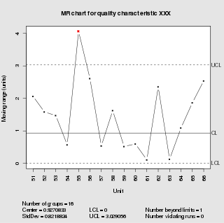
In statistical quality control, the individual/moving-range chart is a type of control chart used to monitor variables data from a business or industrial process for which it is impractical to use rational subgroups.

In statistical quality control, the np-chart is a type of control chart used to monitor the number of nonconforming units in a sample. It is an adaptation of the p-chart and used in situations where personnel find it easier to interpret process performance in terms of concrete numbers of units rather than the somewhat more abstract proportion.
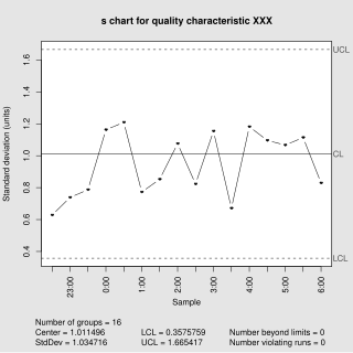
In statistical quality control, the and s chart is a type of control chart used to monitor variables data when samples are collected at regular intervals from a business or industrial process. This is connected to traditional statistical quality control (SQC) and statistical process control (SPC). However, Woodall noted that "I believe that the use of control charts and other monitoring methods should be referred to as “statistical process monitoring,” not “statistical process control (SPC).”"
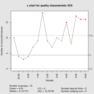
In statistical quality control, the c-chart is a type of control chart used to monitor "count"-type data, typically total number of nonconformities per unit. It is also occasionally used to monitor the total number of events occurring in a given unit of time.

In statistical quality control, an EWMA chart is a type of control chart used to monitor either variables or attributes-type data using the monitored business or industrial process's entire history of output. While other control charts treat rational subgroups of samples individually, the EWMA chart tracks the exponentially-weighted moving average of all prior sample means. EWMA weights samples in geometrically decreasing order so that the most recent samples are weighted most highly while the most distant samples contribute very little.
In survey research, the design effect is a number that shows how well a sample of people may represent a larger group of people for a specific measure of interest. This is important when the sample comes from a sampling method that is different than just picking people using a simple random sample.
Taylor's power law is an empirical law in ecology that relates the variance of the number of individuals of a species per unit area of habitat to the corresponding mean by a power law relationship. It is named after the ecologist who first proposed it in 1961, Lionel Roy Taylor (1924–2007). Taylor's original name for this relationship was the law of the mean. The name Taylor's law was coined by Southwood in 1966.
In statistics, a variables sampling plan is an acceptance sampling technique. Plans for variables are intended for quality characteristics that are measured on a continuous scale. This plan requires the knowledge of the statistical model. The historical evolution of this technique dates back to the seminal work of W. Allen Wallis (1943). The purpose of a plan for variables is to assess whether the process is operating far enough from the specification limit. Plans for variables may produce a similar OC curve to attribute plans with significantly less sample size.


