Angular momentum operator

In quantum mechanics, the angular momentum operator is one of several related operators analogous to classical angular momentum. The angular momentum operator plays a central role in the theory of atomic and molecular physics and other quantum problems involving rotational symmetry. Such an operator is applied to a mathematical representation of the physical state of a system and yields an angular momentum value if the state has a definite value for it. In both classical and quantum mechanical systems, angular momentum (together with linear momentum and energy) is one of the three fundamental properties of motion. ^[1]

There are several angular momentum operators: total angular momentum (usually denoted J), orbital angular momentum (usually denoted L), and spin angular momentum (spin for short, usually denoted S). The term angular momentum operator can (confusingly) refer to either the total or the orbital angular momentum. Total angular momentum is always conserved, see Noether's theorem.

Overview

"Vector cones" of total angular momentum J (green), orbital L (blue), and spin S (red). The cones arise due to quantum uncertainty between measuring angular momentum components (see below).

In quantum mechanics, angular momentum can refer to one of three different, but related things.

Orbital angular momentum

The classical definition of angular momentum is ${\displaystyle \mathbf {L} =\mathbf {r} \times \mathbf {p} }$. The quantum-mechanical counterparts of these objects share the same relationship:

$${\displaystyle \mathbf {L} =\mathbf {r} \times \mathbf {p} }$$

where r is the quantum position operator, p is the quantum momentum operator, × is cross product, and L is the orbital angular momentum operator. L (just like p and r) is a vector operator (a vector whose components are operators), i.e. ${\displaystyle \mathbf {L} =\left(L_{x},L_{y},L_{z}\right)}$ where L_x, L_y, L_z are three different quantum-mechanical operators.

In the special case of a single particle with no electric charge and no spin, the orbital angular momentum operator can be written in the position basis as:

$${\displaystyle \mathbf {L} =-i\hbar (\mathbf {r} \times \nabla )}$$

where ∇ is the vector differential operator, del.

Spin angular momentum

Main article: Spin (physics)

There is another type of angular momentum, called spin angular momentum (more often shortened to spin), represented by the spin operator ${\displaystyle \mathbf {S} =\left(S_{x},S_{y},S_{z}\right)}$. Spin is often depicted as a particle literally spinning around an axis, but this is only a metaphor: the closest classical analog is based on wave circulation. ^[2] All elementary particles have a characteristic spin (scalar bosons have zero spin). For example, electrons always have "spin 1/2" while photons always have "spin 1" (details below).

Total angular momentum

Finally, there is total angular momentum ${\displaystyle \mathbf {J} =\left(J_{x},J_{y},J_{z}\right)}$, which combines both the spin and orbital angular momentum of a particle or system:

$${\displaystyle \mathbf {J} =\mathbf {L} +\mathbf {S} .}$$

Conservation of angular momentum states that J for a closed system, or J for the whole universe, is conserved. However, L and S are not generally conserved. For example, the spin–orbit interaction allows angular momentum to transfer back and forth between L and S, with the total J remaining constant.

Commutation relations

Commutation relations between components

The orbital angular momentum operator is a vector operator, meaning it can be written in terms of its vector components ${\displaystyle \mathbf {L} =\left(L_{x},L_{y},L_{z}\right)}$. The components have the following commutation relations with each other: ^[3]

$${\displaystyle \left[L_{x},L_{y}\right]=i\hbar L_{z},\;\;\left[L_{y},L_{z}\right]=i\hbar L_{x},\;\;\left[L_{z},L_{x}\right]=i\hbar L_{y},}$$

where [ , ] denotes the commutator

$${\displaystyle [X,Y]\equiv XY-YX.}$$

This can be written generally as

$${\displaystyle \left[L_{l},L_{m}\right]=i\hbar \sum _{n=1}^{3}\varepsilon _{lmn}L_{n},}$$

where l, m, n are the component indices (1 for x, 2 for y, 3 for z), and ε_lmn denotes the Levi-Civita symbol.

A compact expression as one vector equation is also possible: ^[4]

$${\displaystyle \mathbf {L} \times \mathbf {L} =i\hbar \mathbf {L} }$$

The commutation relations can be proved as a direct consequence of the canonical commutation relations ${\displaystyle [x_{l},p_{m}]=i\hbar \delta _{lm}}$, where δ_lm is the Kronecker delta.

There is an analogous relationship in classical physics: ^[5]

$${\displaystyle \left\{L_{i},L_{j}\right\}=\varepsilon _{ijk}L_{k}}$$

where L_n is a component of the classical angular momentum operator, and ${\displaystyle \{,\}}$ is the Poisson bracket.

The same commutation relations apply for the other angular momentum operators (spin and total angular momentum): ^[6]

$${\displaystyle \left[S_{l},S_{m}\right]=i\hbar \sum _{n=1}^{3}\varepsilon _{lmn}S_{n},\quad \left[J_{l},J_{m}\right]=i\hbar \sum _{n=1}^{3}\varepsilon _{lmn}J_{n}.}$$

These can be assumed to hold in analogy with L. Alternatively, they can be derived as discussed below.

These commutation relations mean that L has the mathematical structure of a Lie algebra, and the ε_lmn are its structure constants. In this case, the Lie algebra is SU(2) or SO(3) in physics notation (${\displaystyle \operatorname {su} (2)}$ or ${\displaystyle \operatorname {so} (3)}$ respectively in mathematics notation), i.e. Lie algebra associated with rotations in three dimensions. The same is true of J and S. The reason is discussed below. These commutation relations are relevant for measurement and uncertainty, as discussed further below.

In molecules the total angular momentum F is the sum of the rovibronic (orbital) angular momentum N, the electron spin angular momentum S, and the nuclear spin angular momentum I. For electronic singlet states the rovibronic angular momentum is denoted J rather than N. As explained by Van Vleck, ^[7] the components of the molecular rovibronic angular momentum referred to molecule-fixed axes have different commutation relations from those given above which are for the components about space-fixed axes.

Commutation relations involving vector magnitude

Like any vector, the square of a magnitude can be defined for the orbital angular momentum operator,

$${\displaystyle L^{2}\equiv L_{x}^{2}+L_{y}^{2}+L_{z}^{2}.}$$

${\displaystyle L^{2}}$ is another quantum operator. It commutes with the components of ${\displaystyle \mathbf {L} }$,

$${\displaystyle \left[L^{2},L_{x}\right]=\left[L^{2},L_{y}\right]=\left[L^{2},L_{z}\right]=0.}$$

One way to prove that these operators commute is to start from the [L_ℓ, L_m] commutation relations in the previous section:

Proof of [L², L_x] = 0, starting from the [L_ℓ, L_m] commutation relations ^[8]

$${\displaystyle {\begin{aligned}\left[L^{2},L_{x}\right]&=\left[L_{x}^{2},L_{x}\right]+\left[L_{y}^{2},L_{x}\right]+\left[L_{z}^{2},L_{x}\right]\\&=L_{y}\left[L_{y},L_{x}\right]+\left[L_{y},L_{x}\right]L_{y}+L_{z}\left[L_{z},L_{x}\right]+\left[L_{z},L_{x}\right]L_{z}\\&=L_{y}\left(-i\hbar L_{z}\right)+\left(-i\hbar L_{z}\right)L_{y}+L_{z}\left(i\hbar L_{y}\right)+\left(i\hbar L_{y}\right)L_{z}\\&=0\end{aligned}}}$$

Mathematically, ${\displaystyle L^{2}}$ is a Casimir invariant of the Lie algebra SO(3) spanned by ${\displaystyle \mathbf {L} }$.

As above, there is an analogous relationship in classical physics:

$${\displaystyle \left\{L^{2},L_{x}\right\}=\left\{L^{2},L_{y}\right\}=\left\{L^{2},L_{z}\right\}=0}$$

where ${\displaystyle L_{i}}$ is a component of the classical angular momentum operator, and ${\displaystyle \{,\}}$ is the Poisson bracket. ^[9]

Returning to the quantum case, the same commutation relations apply to the other angular momentum operators (spin and total angular momentum), as well,

$${\displaystyle {\begin{aligned}\left[S^{2},S_{i}\right]&=0,\\\left[J^{2},J_{i}\right]&=0.\end{aligned}}}$$

Uncertainty principle

Main articles: Uncertainty principle and Uncertainty principle derivations

In general, in quantum mechanics, when two observable operators do not commute, they are called complementary observables. Two complementary observables cannot be measured simultaneously; instead they satisfy an uncertainty principle. The more accurately one observable is known, the less accurately the other one can be known. Just as there is an uncertainty principle relating position and momentum, there are uncertainty principles for angular momentum.

The Robertson–Schrödinger relation gives the following uncertainty principle:

$${\displaystyle \sigma _{L_{x}}\sigma _{L_{y}}\geq {\frac {\hbar }{2}}\left|\langle L_{z}\rangle \right|.}$$

where ${\displaystyle \sigma _{X}}$ is the standard deviation in the measured values of X and ${\displaystyle \langle X\rangle }$ denotes the expectation value of X. This inequality is also true if x, y, z are rearranged, or if L is replaced by J or S.

Therefore, two orthogonal components of angular momentum (for example L_x and L_y) are complementary and cannot be simultaneously known or measured, except in special cases such as ${\displaystyle L_{x}=L_{y}=L_{z}=0}$.

It is, however, possible to simultaneously measure or specify L² and any one component of L; for example, L² and L_z. This is often useful, and the values are characterized by the azimuthal quantum number (l) and the magnetic quantum number (m). In this case the quantum state of the system is a simultaneous eigenstate of the operators L² and L_z, but not of L_x or L_y. The eigenvalues are related to l and m, as shown in the table below.

Quantization

See also: Azimuthal quantum number and Magnetic quantum number

In quantum mechanics, angular momentum is quantized – that is, it cannot vary continuously, but only in "quantum leaps" between certain allowed values. For any system, the following restrictions on measurement results apply, where ${\displaystyle \hbar }$ is reduced Planck constant: ^[10]

If you measure...	...the result can be...	Notes
${\displaystyle L^{2}}$	${\displaystyle \hbar ^{2}\ell (\ell +1)}$,    where ${\displaystyle \ell =0,1,2,\ldots }$	${\displaystyle \ell }$ is sometimes called azimuthal quantum number or orbital quantum number.
${\displaystyle L_{z}}$	${\displaystyle \hbar m_{\ell }}$,    where ${\displaystyle m_{\ell }=-\ell ,(-\ell +1),\ldots ,(\ell -1),\ell }$	${\displaystyle m_{\ell }}$ is sometimes called magnetic quantum number . This same quantization rule holds for any component of ${\displaystyle \mathbf {L} }$; e.g., ${\displaystyle L_{x}\,or\,L_{y}}$. This rule is sometimes called spatial quantization. [11]
${\displaystyle S^{2}}$	${\displaystyle \hbar ^{2}s(s+1)}$,    where ${\displaystyle s=0,{\tfrac {1}{2}},1,{\tfrac {3}{2}},\ldots }$	s is called spin quantum number or just spin. For example, a spin-1⁄2 particle is a particle where s = 1⁄2.
${\displaystyle S_{z}}$	${\displaystyle \hbar m_{s}}$,    where ${\displaystyle m_{s}=-s,(-s+1),\ldots ,(s-1),s}$	${\displaystyle m_{s}}$ is sometimes called spin projection quantum number . This same quantization rule holds for any component of ${\displaystyle \mathbf {S} }$; e.g., ${\displaystyle S_{x}\,or\,S_{y}}$.
${\displaystyle J^{2}}$	${\displaystyle \hbar ^{2}j(j+1)}$,    where ${\displaystyle j=0,{\tfrac {1}{2}},1,{\tfrac {3}{2}},\ldots }$	j is sometimes called total angular momentum quantum number .
${\displaystyle J_{z}}$	${\displaystyle \hbar m_{j}}$,    where ${\displaystyle m_{j}=-j,(-j+1),\ldots ,(j-1),j}$	${\displaystyle m_{j}}$ is sometimes called total angular momentum projection quantum number . This same quantization rule holds for any component of ${\displaystyle \mathbf {J} }$; e.g., ${\displaystyle J_{x}\,or\,J_{y}}$.

Derivation using ladder operators

Main article: Ladder operator § Angular momentum

A common way to derive the quantization rules above is the method of ladder operators . ^[12] The ladder operators for the total angular momentum ${\displaystyle \mathbf {J} =\left(J_{x},J_{y},J_{z}\right)}$ are defined as:

$${\displaystyle {\begin{aligned}J_{+}&\equiv J_{x}+iJ_{y},\\J_{-}&\equiv J_{x}-iJ_{y}\end{aligned}}}$$

Suppose ${\displaystyle |\psi \rangle }$ is a simultaneous eigenstate of ${\displaystyle J^{2}}$ and ${\displaystyle J_{z}}$ (i.e., a state with a definite value for ${\displaystyle J^{2}}$ and a definite value for ${\displaystyle J_{z}}$). Then using the commutation relations for the components of ${\displaystyle \mathbf {J} }$, one can prove that each of the states ${\displaystyle J_{+}|\psi \rangle }$ and ${\displaystyle J_{-}|\psi \rangle }$ is either zero or a simultaneous eigenstate of ${\displaystyle J^{2}}$ and ${\displaystyle J_{z}}$, with the same value as ${\displaystyle |\psi \rangle }$ for ${\displaystyle J^{2}}$ but with values for ${\displaystyle J_{z}}$ that are increased or decreased by ${\displaystyle \hbar }$ respectively. The result is zero when the use of a ladder operator would otherwise result in a state with a value for ${\displaystyle J_{z}}$ that is outside the allowable range. Using the ladder operators in this way, the possible values and quantum numbers for ${\displaystyle J^{2}}$ and ${\displaystyle J_{z}}$ can be found.

Derivation of the possible values and quantum numbers for ${\displaystyle J_{z}}$ and ${\displaystyle J^{2}}$. ^[13]

Let ${\displaystyle \psi ({J^{2}}'J_{z}')}$ be a state function for the system with eigenvalue ${\displaystyle {J^{2}}'}$ for ${\displaystyle J^{2}}$ and eigenvalue ${\displaystyle J_{z}'}$ for ${\displaystyle J_{z}}$. ^{[note 1]}

From ${\displaystyle J^{2}=J_{x}^{2}+J_{y}^{2}+J_{z}^{2}}$ is obtained,

$${\displaystyle J_{x}^{2}+J_{y}^{2}=J^{2}-J_{z}^{2}.}$$

Applying both sides of the above equation to ${\displaystyle \psi ({J^{2}}'J_{z}')}$,

$${\displaystyle (J_{x}^{2}+J_{y}^{2})\;\psi ({J^{2}}'J_{z}')=({J^{2}}'-J_{z}'^{2})\;\psi ({J^{2}}'J_{z}').}$$

Since ${\displaystyle J_{x}}$ and ${\displaystyle J_{y}}$ are real observables, ${\displaystyle {J^{2}}'-J_{z}'^{2}}$ is not negative and ${\textstyle |J_{z}'|\leq {\sqrt {{J^{2}}'}}}$. Thus ${\displaystyle J_{z}'}$ has an upper and lower bound.

Two of the commutation relations for the components of ${\displaystyle \mathbf {J} }$ are,

$${\displaystyle [J_{y},J_{z}]=i\hbar J_{x},\;\;[J_{z},J_{x}]=i\hbar J_{y}.}$$

They can be combined to obtain two equations, which are written together using ${\displaystyle \pm }$ signs in the following,

$${\displaystyle J_{z}(J_{x}\pm iJ_{y})=(J_{x}\pm iJ_{y})(J_{z}\pm \hbar ),}$$

where one of the equations uses the ${\displaystyle +}$ signs and the other uses the ${\displaystyle -}$ signs. Applying both sides of the above to ${\displaystyle \psi ({J^{2}}'J_{z}')}$,

$${\displaystyle {\begin{aligned}J_{z}(J_{x}\pm iJ_{y})\;\psi ({J^{2}}'J_{z}')&=(J_{x}\pm iJ_{y})(J_{z}\pm \hbar )\;\psi ({J^{2}}'J_{z}')\\&=(J_{z}'\pm \hbar )(J_{x}\pm iJ_{y})\;\psi ({J^{2}}'J_{z}')\;.\\\end{aligned}}}$$

The above shows that ${\displaystyle (J_{x}\pm iJ_{y})\;\psi ({J^{2}}'J_{z}')}$ are two eigenfunctions of ${\displaystyle J_{z}}$ with respective eigenvalues ${\displaystyle {J_{z}}'\pm \hbar }$ , unless one of the functions is zero, in which case it is not an eigenfunction. For the functions that are not zero,

$${\displaystyle \psi ({J^{2}}'J_{z}'\pm \hbar )=(J_{x}\pm iJ_{y})\;\psi ({J^{2}}'J_{z}').}$$

Further eigenfunctions of ${\displaystyle J_{z}}$ and corresponding eigenvalues can be found by repeatedly applying ${\displaystyle J_{x}\pm iJ_{y}}$ as long as the magnitude of the resulting eigenvalue is ${\displaystyle \leq {\sqrt {{J^{2}}'}}}$. Since the eigenvalues of ${\displaystyle J_{z}}$ are bounded, let ${\displaystyle J_{z}^{0}}$ be the lowest eigenvalue and ${\displaystyle J_{z}^{1}}$ be the highest. Then

$${\displaystyle (J_{x}-iJ_{y})\;\psi ({J^{2}}'J_{z}^{0})=0}$$

and

$${\displaystyle (J_{x}+iJ_{y})\;\psi ({J^{2}}'J_{z}^{1})=0,}$$

since there are no states where the eigenvalue of ${\displaystyle J_{z}}$ is ${\displaystyle <J_{z}^{0}}$ or ${\displaystyle >J_{z}^{1}}$. By applying ${\displaystyle (J_{x}+iJ_{y})}$ to the first equation, ${\displaystyle (J_{x}-iJ_{y})}$ to the second, and using ${\displaystyle J_{x}^{2}+J_{y}^{2}=J^{2}-J_{z}^{2}}$, it can be shown that

$${\displaystyle {J^{2}}'-(J_{z}^{0})^{2}+\hbar J_{z}^{0}=0}$$

and

$${\displaystyle {J^{2}}'-(J_{z}^{1})^{2}-\hbar J_{z}^{1}=0.}$$

Subtracting the first equation from the second and rearranging,

$${\displaystyle (J_{z}^{1}+J_{z}^{0})(J_{z}^{0}-J_{z}^{1}-\hbar )=0.}$$

Since ${\displaystyle J_{z}^{1}\geq J_{z}^{0}}$, the second factor is negative. Then the first factor must be zero and thus ${\displaystyle J_{z}^{0}=-J_{z}^{1}}$.

The difference ${\displaystyle J_{z}^{1}-J_{z}^{0}}$ comes from successive application of ${\displaystyle J_{x}-iJ_{y}}$ or ${\displaystyle J_{x}+iJ_{y}}$ which lower or raise the eigenvalue of ${\displaystyle J_{z}}$ by ${\displaystyle \hbar }$ so that,

$${\displaystyle J_{z}^{1}-J_{z}^{0}=0,\hbar ,2\hbar ,\dots }$$

Let

$${\displaystyle J_{z}^{1}-J_{z}^{0}=2j\hbar ,}$$

where

$${\displaystyle j=0,{\tfrac {1}{2}},1,{\tfrac {3}{2}},\dots \;.}$$

Then using ${\displaystyle J_{z}^{0}=-J_{z}^{1}}$ and the above,

$${\displaystyle J_{z}^{0}=-j\hbar }$$

and

$${\displaystyle J_{z}^{1}=j\hbar ,}$$

and the allowable eigenvalues of ${\displaystyle J_{z}}$ are

$${\displaystyle J_{z}'=-j\hbar ,-j\hbar +\hbar ,-j\hbar +2\hbar ,\dots ,j\hbar .}$$

Expressing ${\displaystyle J_{z}'}$ in terms of a quantum number ${\displaystyle m_{j}\;}$, and substituting ${\displaystyle J_{z}^{0}=-j\hbar }$ into ${\displaystyle {J^{2}}'-(J_{z}^{0})^{2}+\hbar J_{z}^{0}=0}$ from above,

${\displaystyle {\begin{aligned}J_{z}'&=m_{j}\hbar &m_{j}&=-j,-j+1,-j+2,\dots ,j\\{J^{2}}'&=j(j+1)\hbar ^{2}&j&=0,{\tfrac {1}{2}},1,{\tfrac {3}{2}},\dots \;.\end{aligned}}}$

Since ${\displaystyle \mathbf {S} }$ and ${\displaystyle \mathbf {L} }$ have the same commutation relations as ${\displaystyle \mathbf {J} }$, the same ladder analysis can be applied to them, except that for ${\displaystyle \mathbf {L} }$ there is a further restriction on the quantum numbers that they must be integers.

Traditional derivation of the restriction to integer quantum numbers for ${\displaystyle L_{z}}$ and ${\displaystyle L^{2}}$. ^[14]

In the Schroedinger representation, the z component of the orbital angular momentum operator can be expressed in spherical coordinates as, ^[15]

$${\displaystyle L_{z}=-i\hbar {\frac {\partial }{\partial \phi }}.}$$

For ${\displaystyle L_{z}}$ and eigenfunction ${\displaystyle \psi }$ with eigenvalue ${\displaystyle L_{z}'}$,

$${\displaystyle -i\hbar {\frac {\partial }{\partial \phi }}\psi =L_{z}'\psi .}$$

Solving for ${\displaystyle \psi }$,

$${\displaystyle \psi =Ae^{iL_{z}'\phi /\hbar },}$$

where ${\displaystyle A}$ is independent of ${\displaystyle \phi }$. Since ${\displaystyle \psi }$ is required to be single valued, and adding ${\displaystyle 2\pi }$ to ${\displaystyle \phi }$ results in a coordinate for the same point in space,

$${\displaystyle {\begin{aligned}Ae^{iL_{z}'(\phi +2\pi )/\hbar }&=Ae^{iL_{z}'\phi /\hbar },\\e^{iL_{z}'2\pi /\hbar }&=1.\end{aligned}}}$$

Solving for the eigenvalue ${\displaystyle L_{z}'}$,

$${\displaystyle L_{z}'=m_{l}\hbar \;,}$$

where ${\displaystyle m_{l}}$ is an integer. ^[16] From the above and the relation ${\displaystyle m_{\ell }=-\ell ,(-\ell +1),\ldots ,(\ell -1),\ell \ \ }$, it follows that ${\displaystyle \ell }$ is also an integer. This shows that the quantum numbers ${\displaystyle m_{\ell }}$ and ${\displaystyle \ell }$ for the orbital angular momentum ${\displaystyle \mathbf {L} }$ are restricted to integers, unlike the quantum numbers for the total angular momentum ${\displaystyle \mathbf {J} }$ and spin ${\displaystyle \mathbf {S} }$, which can have half-integer values. ^[17]

An alternative derivation which does not assume single-valued wave functions follows and another argument using Lie groups is below.

Alternative derivation of the restriction to integer quantum numbers for ${\displaystyle L_{z}}$ and ${\displaystyle L^{2}}$

A key part of the traditional derivation above is that the wave function must be single-valued. This is now recognised by many as not being completely correct: a wave function ${\displaystyle \psi }$ is not observable and only the probability density ${\displaystyle \psi ^{*}\psi }$ is required to be single-valued. The possible double-valued half-integer wave functions have a single-valued probability density. ^[18] This was recognised by Pauli in 1939 (cited by Japaridze et al ^[19] )

... there is no a priori convincing argument stating that the wave functions which describe some physical states must be single valued functions. For physical quantities, which are expressed by squares of wave functions, to be single valued it is quite sufficient that after moving around a closed contour these functions gain a factor exp(iα)

Double-valued wave functions have been found, such as ${\displaystyle \left|{\tfrac {1}{2}},{\tfrac {1}{2}}\right\rangle =e^{i\phi /2}\sin ^{\frac {1}{2}}\theta }$ and ${\displaystyle \left|{\tfrac {1}{2}},-{\tfrac {1}{2}}\right\rangle =e^{-i\phi /2}\sin ^{\frac {1}{2}}\theta }$. ^{[20] [21]} These do not behave well under the ladder operators, but have been found to be useful in describing rigid quantum particles ^[22]

Ballentine ^[23] gives an argument based solely on the operator formalism and which does not rely on the wave function being single-valued. The azimuthal angular momentum is defined as

$${\displaystyle L_{z}=Q_{x}P_{y}-Q_{y}P_{x}}$$

Define new operators

$${\displaystyle {\begin{aligned}q_{1}&={\frac {Q_{x}+P_{y}}{\sqrt {2}}}&q_{2}&={\frac {Q_{x}-P_{y}}{\sqrt {2}}}\\p_{1}&={\frac {P_{x}-Q_{y}}{\sqrt {2}}}&p_{2}&={\frac {P_{x}+Q_{y}}{\sqrt {2}}}\end{aligned}}}$$

(Dimensional correctness may be maintained by inserting factors of mass and unit angular frequency numerically equal to one.) Then

$${\displaystyle L_{z}={\tfrac {1}{2}}\left(p_{1}^{2}+q_{1}^{2}\right)-{\tfrac {1}{2}}\left(p_{2}^{2}+q_{2}^{2}\right)}$$

But the two terms on the right are just the Hamiltonians for the quantum harmonic oscillator with unit mass and angular frequency

$${\displaystyle {\begin{aligned}H_{1}&={\tfrac {1}{2}}\left(p_{1}^{2}+q_{1}^{2}\right)\\H_{2}&={\tfrac {1}{2}}\left(p_{2}^{2}+q_{2}^{2}\right)\end{aligned}}}$$

and ${\displaystyle L^{2}}$, ${\displaystyle L_{z}}$, ${\displaystyle H_{1}}$ and ${\displaystyle H_{2}}$ all commute.

For commuting Hermitian operators a complete set of basis vectors can be chosen that are eigenvectors for all four operators. (The argument by Glorioso ^[24] can easily be generalised to any number of commuting operators.)

For any of these eigenvectors ${\displaystyle \psi }$ with

$${\displaystyle {\begin{aligned}L^{2}\psi &=\hbar ^{2}\ell (\ell +1)\psi \\L_{z}\psi &=\hbar m\psi \\H_{1}\psi &=\hbar \left(n_{1}+{\tfrac {1}{2}}\right)\psi \\H_{2}\psi &=\hbar \left(n_{2}+{\tfrac {1}{2}}\right)\psi \end{aligned}}}$$

for some integers ${\displaystyle n_{1},n_{2}}$, we find

$${\displaystyle m=\left(n_{1}+{\tfrac {1}{2}}\right)-\left(n_{2}+{\tfrac {1}{2}}\right)=n_{1}-n_{2}}$$

As a difference of two integers, ${\displaystyle m}$ must be an integer, from which ${\displaystyle \ell }$ is also integral.

A more complex version of this argument using the ladder operators of the quantum harmonic oscillator has been given by Buchdahl. ^[25]

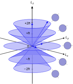
Visual interpretation

Illustration of the vector model of orbital angular momentum.

Since the angular momenta are quantum operators, they cannot be drawn as vectors like in classical mechanics. Nevertheless, it is common to depict them heuristically in this way. Depicted on the right is a set of states with quantum numbers ${\displaystyle \ell =2}$, and ${\displaystyle m_{\ell }=-2,-1,0,1,2}$ for the five cones from bottom to top. Since ${\displaystyle |L|={\sqrt {L^{2}}}=\hbar {\sqrt {6}}}$, the vectors are all shown with length ${\displaystyle \hbar {\sqrt {6}}}$. The rings represent the fact that ${\displaystyle L_{z}}$ is known with certainty, but ${\displaystyle L_{x}}$ and ${\displaystyle L_{y}}$ are unknown; therefore every classical vector with the appropriate length and z-component is drawn, forming a cone. The expected value of the angular momentum for a given ensemble of systems in the quantum state characterized by ${\displaystyle \ell }$ and ${\displaystyle m_{\ell }}$ could be somewhere on this cone while it cannot be defined for a single system (since the components of ${\displaystyle L}$ do not commute with each other).

Quantization in macroscopic systems

The quantization rules are widely thought to be true even for macroscopic systems, like the angular momentum L of a spinning tire. However they have no observable effect so this has not been tested. For example, if ${\displaystyle L_{z}/\hbar }$ is roughly 100000000, it makes essentially no difference whether the precise value is an integer like 100000000 or 100000001, or a non-integer like 100000000.2—the discrete steps are currently too small to measure.

Angular momentum as the generator of rotations

See also: Total angular momentum quantum number

The most general and fundamental definition of angular momentum is as the generator of rotations. ^[6] More specifically, let ${\displaystyle R({\hat {n}},\phi )}$ be a rotation operator, which rotates any quantum state about axis ${\displaystyle {\hat {n}}}$ by angle ${\displaystyle \phi }$. As ${\displaystyle \phi \rightarrow 0}$, the operator ${\displaystyle R({\hat {n}},\phi )}$ approaches the identity operator, because a rotation of 0° maps all states to themselves. Then the angular momentum operator ${\displaystyle J_{\hat {n}}}$ about axis ${\displaystyle {\hat {n}}}$ is defined as: ^[6]

$${\displaystyle J_{\hat {n}}\equiv i\hbar \lim _{\phi \rightarrow 0}{\frac {R\left({\hat {n}},\phi \right)-1}{\phi }}=\left.i\hbar {\frac {\partial R\left({\hat {n}},\phi \right)}{\partial \phi }}\right|_{\phi =0}}$$

where 1 is the identity operator. Also notice that R is an additive morphism : ${\displaystyle R\left({\hat {n}},\phi _{1}+\phi _{2}\right)=R\left({\hat {n}},\phi _{1}\right)R\left({\hat {n}},\phi _{2}\right)}$ ; as a consequence ^[6]

$${\displaystyle R\left({\hat {n}},\phi \right)=\exp \left(-{\frac {i\phi J_{\hat {n}}}{\hbar }}\right)}$$

where exp is matrix exponential. The existence of the generator is guaranteed by the Stone's theorem on one-parameter unitary groups.

In simpler terms, the total angular momentum operator characterizes how a quantum system is changed when it is rotated. The relationship between angular momentum operators and rotation operators is the same as the relationship between Lie algebras and Lie groups in mathematics, as discussed further below.

The different types of rotation operators. The top box shows two particles, with spin states indicated schematically by the arrows.

1. The operator R, related to J, rotates the entire system.
2. The operator R_spatial, related to L, rotates the particle positions without altering their internal spin states.
3. The operator R_internal, related to S, rotates the particles' internal spin states without changing their positions.

Just as J is the generator for rotation operators, L and S are generators for modified partial rotation operators. The operator

$${\displaystyle R_{\text{spatial}}\left({\hat {n}},\phi \right)=\exp \left(-{\frac {i\phi L_{\hat {n}}}{\hbar }}\right),}$$

rotates the position (in space) of all particles and fields, without rotating the internal (spin) state of any particle. Likewise, the operator

$${\displaystyle R_{\text{internal}}\left({\hat {n}},\phi \right)=\exp \left(-{\frac {i\phi S_{\hat {n}}}{\hbar }}\right),}$$

rotates the internal (spin) state of all particles, without moving any particles or fields in space. The relation J = L + S comes from:

$${\displaystyle R\left({\hat {n}},\phi \right)=R_{\text{internal}}\left({\hat {n}},\phi \right)R_{\text{spatial}}\left({\hat {n}},\phi \right)}$$

i.e. if the positions are rotated, and then the internal states are rotated, then altogether the complete system has been rotated.

SU(2), SO(3), and 360° rotations

Main article: Spin (physics)

Although one might expect ${\displaystyle R\left({\hat {n}},360^{\circ }\right)=1}$ (a rotation of 360° is the identity operator), this is not assumed in quantum mechanics, and it turns out it is often not true: When the total angular momentum quantum number is a half-integer (1/2, 3/2, etc.), ${\displaystyle R\left({\hat {n}},360^{\circ }\right)=-1}$, and when it is an integer, ${\displaystyle R\left({\hat {n}},360^{\circ }\right)=+1}$. ^[6] Mathematically, the structure of rotations in the universe is not SO(3), the group of three-dimensional rotations in classical mechanics. Instead, it is SU(2), which is identical to SO(3) for small rotations, but where a 360° rotation is mathematically distinguished from a rotation of 0°. (A rotation of 720° is, however, the same as a rotation of 0°.) ^[6]

On the other hand, ${\displaystyle R_{\text{spatial}}\left({\hat {n}},360^{\circ }\right)=+1}$ in all circumstances, because a 360° rotation of a spatial configuration is the same as no rotation at all. (This is different from a 360° rotation of the internal (spin) state of the particle, which might or might not be the same as no rotation at all.) In other words, the ${\displaystyle R_{\text{spatial}}}$ operators carry the structure of SO(3), while ${\displaystyle R}$ and ${\displaystyle R_{\text{internal}}}$ carry the structure of SU(2).

From the equation ${\displaystyle +1=R_{\text{spatial}}\left({\hat {z}},360^{\circ }\right)=\exp \left(-2\pi iL_{z}/\hbar \right)}$, one picks an eigenstate ${\displaystyle L_{z}|\psi \rangle =m\hbar |\psi \rangle }$ and draws

$${\displaystyle e^{-2\pi im}=1}$$

which is to say that the orbital angular momentum quantum numbers can only be integers, not half-integers.

Connection to representation theory

Main articles: Particle physics and representation theory, Representation theory of SU(2), and Rotation group SO(3) § A note on Lie algebras

Starting with a certain quantum state ${\displaystyle |\psi _{0}\rangle }$, consider the set of states ${\displaystyle R\left({\hat {n}},\phi \right)\left|\psi _{0}\right\rangle }$ for all possible ${\displaystyle {\hat {n}}}$ and ${\displaystyle \phi }$, i.e. the set of states that come about from rotating the starting state in every possible way. The linear span of that set is a vector space, and therefore the manner in which the rotation operators map one state onto another is a representation of the group of rotation operators.

When rotation operators act on quantum states, it forms a representation of the Lie group SU(2) (for R and R_internal), or SO(3) (for R_spatial).

From the relation between J and rotation operators,

When angular momentum operators act on quantum states, it forms a representation of the Lie algebra ${\displaystyle {\mathfrak {su}}(2)}$ or ${\displaystyle {\mathfrak {so}}(3)}$.

(The Lie algebras of SU(2) and SO(3) are identical.)

The ladder operator derivation above is a method for classifying the representations of the Lie algebra SU(2).

Connection to commutation relations

Classical rotations do not commute with each other: For example, rotating 1° about the x-axis then 1° about the y-axis gives a slightly different overall rotation than rotating 1° about the y-axis then 1° about the x-axis. By carefully analyzing this noncommutativity, the commutation relations of the angular momentum operators can be derived. ^[6]

(This same calculational procedure is one way to answer the mathematical question "What is the Lie algebra of the Lie groups SO(3) or SU(2)?")

Conservation of angular momentum

The Hamiltonian H represents the energy and dynamics of the system. In a spherically symmetric situation, the Hamiltonian is invariant under rotations:

$${\displaystyle RHR^{-1}=H}$$

where R is a rotation operator. As a consequence, ${\displaystyle [H,R]=0}$, and then ${\displaystyle [H,\mathbf {J} ]=\mathbf {0} }$ due to the relationship between J and R. By the Ehrenfest theorem, it follows that J is conserved.

To summarize, if H is rotationally-invariant (spherically symmetric), then total angular momentum J is conserved. This is an example of Noether's theorem.

If H is just the Hamiltonian for one particle, the total angular momentum of that one particle is conserved when the particle is in a central potential (i.e., when the potential energy function depends only on ${\displaystyle \left|\mathbf {r} \right|}$). Alternatively, H may be the Hamiltonian of all particles and fields in the universe, and then H is always rotationally-invariant, as the fundamental laws of physics of the universe are the same regardless of orientation. This is the basis for saying conservation of angular momentum is a general principle of physics.

For a particle without spin, J = L, so orbital angular momentum is conserved in the same circumstances. When the spin is nonzero, the spin–orbit interaction allows angular momentum to transfer from L to S or back. Therefore, L is not, on its own, conserved.

Angular momentum coupling

Main articles: Angular momentum coupling and Clebsch–Gordan coefficients

Often, two or more sorts of angular momentum interact with each other, so that angular momentum can transfer from one to the other. For example, in spin–orbit coupling, angular momentum can transfer between L and S, but only the total J = L + S is conserved. In another example, in an atom with two electrons, each has its own angular momentum J₁ and J₂, but only the total J = J₁ + J₂ is conserved.

In these situations, it is often useful to know the relationship between, on the one hand, states where ${\displaystyle \left(J_{1}\right)_{z},\left(J_{1}\right)^{2},\left(J_{2}\right)_{z},\left(J_{2}\right)^{2}}$ all have definite values, and on the other hand, states where ${\displaystyle \left(J_{1}\right)^{2},\left(J_{2}\right)^{2},J^{2},J_{z}}$ all have definite values, as the latter four are usually conserved (constants of motion). The procedure to go back and forth between these bases is to use Clebsch–Gordan coefficients.

One important result in this field is that a relationship between the quantum numbers for ${\displaystyle \left(J_{1}\right)^{2},\left(J_{2}\right)^{2},J^{2}}$:

$${\displaystyle j\in \left\{\left|j_{1}-j_{2}\right|,\left(\left|j_{1}-j_{2}\right|+1\right),\ldots ,\left(j_{1}+j_{2}\right)\right\}.}$$

For an atom or molecule with J = L + S, the term symbol gives the quantum numbers associated with the operators ${\displaystyle L^{2},S^{2},J^{2}}$.

Orbital angular momentum in spherical coordinates

Angular momentum operators usually occur when solving a problem with spherical symmetry in spherical coordinates. The angular momentum in the spatial representation is ^{[26] [27]}

$${\displaystyle {\begin{aligned}\mathbf {L} &=i\hbar \left({\frac {\hat {\boldsymbol {\theta }}}{\sin(\theta )}}{\frac {\partial }{\partial \phi }}-{\hat {\boldsymbol {\phi }}}{\frac {\partial }{\partial \theta }}\right)\\&=i\hbar \left({\hat {\mathbf {x} }}\left(\sin(\phi ){\frac {\partial }{\partial \theta }}+\cot(\theta )\cos(\phi ){\frac {\partial }{\partial \phi }}\right)+{\hat {\mathbf {y} }}\left(-\cos(\phi ){\frac {\partial }{\partial \theta }}+\cot(\theta )\sin(\phi ){\frac {\partial }{\partial \phi }}\right)-{\hat {\mathbf {z} }}{\frac {\partial }{\partial \phi }}\right)\\L_{+}&=\hbar e^{i\phi }\left({\frac {\partial }{\partial \theta }}+i\cot(\theta ){\frac {\partial }{\partial \phi }}\right),\\L_{-}&=\hbar e^{-i\phi }\left(-{\frac {\partial }{\partial \theta }}+i\cot(\theta ){\frac {\partial }{\partial \phi }}\right),\\L^{2}&=-\hbar ^{2}\left({\frac {1}{\sin(\theta )}}{\frac {\partial }{\partial \theta }}\left(\sin(\theta ){\frac {\partial }{\partial \theta }}\right)+{\frac {1}{\sin ^{2}(\theta )}}{\frac {\partial ^{2}}{\partial \phi ^{2}}}\right),\\L_{z}&=-i\hbar {\frac {\partial }{\partial \phi }}.\end{aligned}}}$$

In spherical coordinates the angular part of the Laplace operator can be expressed by the angular momentum. This leads to the relation

$${\displaystyle \Delta ={\frac {1}{r^{2}}}{\frac {\partial }{\partial r}}\left(r^{2}\,{\frac {\partial }{\partial r}}\right)-{\frac {L^{2}}{\hbar ^{2}r^{2}}}.}$$

When solving to find eigenstates of the operator ${\displaystyle L^{2}}$, we obtain the following

$${\displaystyle {\begin{aligned}L^{2}\left|\ell ,m\right\rangle &=\hbar ^{2}\ell (\ell +1)\left|\ell ,m\right\rangle \\L_{z}\left|\ell ,m\right\rangle &=\hbar m\left|\ell ,m\right\rangle \end{aligned}}}$$

where

$${\displaystyle \left\langle \theta ,\phi |\ell ,m\right\rangle =Y_{\ell ,m}(\theta ,\phi )}$$

are the spherical harmonics. ^[28]

See also

• Runge–Lenz vector (used to describe the shape and orientation of bodies in orbit)
• Holstein–Primakoff transformation
• Jordan map (Schwinger's bosonic model of angular momentum ^[29] )
• Pauli–Lubanski pseudovector
• Angular momentum diagrams (quantum mechanics)
• Spherical basis
• Tensor operator
• Orbital magnetization
• Orbital angular momentum of free electrons
• Orbital angular momentum of light

Notes

1. In the derivation of Condon and Shortley that the current derivation is based on, a set of observables ${\displaystyle \Gamma }$ along with ${\displaystyle J^{2}}$ and ${\displaystyle J_{z}}$ form a complete set of commuting observables. Additionally they required that ${\displaystyle \Gamma }$ commutes with ${\displaystyle J_{x}}$ and ${\displaystyle J_{y}}$. ^[13] The present derivation is simplified by not including the set ${\displaystyle \Gamma }$ or its corresponding set of eigenvalues ${\displaystyle \gamma }$.

References

1. Introductory Quantum Mechanics, Richard L. Liboff, 2nd Edition, ISBN   0-201-54715-5
2. Ohanian, Hans C. (1986-06-01). "What is spin?" (PDF). American Journal of Physics. 54 (6): 500–505. Bibcode:1986AmJPh..54..500O. doi:10.1119/1.14580. ISSN   0002-9505.
3. Aruldhas, G. (2004-02-01). "formula (8.8)". Quantum Mechanics. Prentice Hall India. p. 171. ISBN   978-81-203-1962-2.
4. Shankar, R. (1994). Principles of quantum mechanics (2nd ed.). New York: Kluwer Academic / Plenum. p.  319. ISBN   9780306447907.
5. H. Goldstein, C. P. Poole and J. Safko, Classical Mechanics, 3rd Edition, Addison-Wesley 2002, pp. 388 ff.
6. Littlejohn, Robert (2011). "Lecture notes on rotations in quantum mechanics" (PDF). Physics 221B Spring 2011. Archived from the original (PDF) on 26 August 2014. Retrieved 13 Jan 2012.
7. J. H. Van Vleck (1951). "The Coupling of Angular Momentum Vectors in Molecules". Reviews of Modern Physics. 23 (3): 213. Bibcode:1951RvMP...23..213V. doi:10.1103/RevModPhys.23.213.
8. Griffiths, David J. (1995). Introduction to Quantum Mechanics . Prentice Hall. p.  146.
9. Goldstein et al, p. 410
10. Condon, E. U.; Shortley, G. H. (1935). "Chapter III: Angular Momentum". Quantum Theory of Atomic Spectra. Cambridge University Press. ISBN   9780521092098.
11. Introduction to quantum mechanics: with applications to chemistry, by Linus Pauling, Edgar Bright Wilson, page 45, google books link
12. Griffiths, David J. (1995). Introduction to Quantum Mechanics . Prentice Hall. pp.  147–149.
13. Condon & Shortley 1935, pp.  46–47
14. Condon & Shortley 1935, pp.  50–51
15. Condon & Shortley 1935, p. 50, Eq 1
16. Condon & Shortley 1935, p. 50, Eq 3
17. Condon & Shortley 1935, p. 51
18. Ballentine, L. E. (1998). Quantum Mechanics: A Modern Development. World Scientific Publishing. p. 169.
19. Japaridze, G.; Khelashvili, A.; Turashvili, K. (2020). "Critical comments on the quantization of the angular momentum: II. Analysis based on the requirement that the eigenfunction of the third component of the operator of the angular momentum must be a single valued periodic function". arXiv: 2004.10673 [physics.gen-ph].
20. Hunter, G.; et al. (1999). "Fermion quasi-spherical harmonics". Journal of Physics A. 32 (5): 795–803. arXiv: math-ph/9810001 . Bibcode:1999JPhA...32..795H. doi:10.1088/0305-4470/32/5/011. S2CID   119721724.
21. Hunter, G.; I., Schlifer (2008). "Explicit Spin Coordinates". arXiv: quant-ph/0507008 .
22. Pavšič, M (2007). "Rigid Particle and its Spin Revisited". Foundations of Physics. 37 (1): 40–79. arXiv: hep-th/0412324 . Bibcode:2007FoPh...37...40P. doi:10.1007/s10701-006-9094-4. S2CID   119648904.
23. Ballentine, L. E. (1998). Quantum Mechanics: A Modern Development. World Scientific Publishing. pp. 169–171.
24. Glorioso, P. "On common eigenbases of commuting operators" (PDF). Retrieved 14 August 2021.
25. Buchdahl, H. A. (1962). "Remark Concerning the Eigenvalues of Orbital Angular Momentum". American Journal of Physics. 30 (11): 829–831. Bibcode:1962AmJPh..30..829B. doi:10.1119/1.1941817.
26. Bes, Daniel R. (2007). Quantum Mechanics. Advanced Texts in Physics. Berlin, Heidelberg: Springer Berlin Heidelberg. p. 70. Bibcode:2007qume.book.....B. doi:10.1007/978-3-540-46216-3. ISBN   978-3-540-46215-6.
27. Compare and contrast with the contragredient classical L.
28. Sakurai, JJ & Napolitano, J (2010), Modern Quantum Mechanics (2nd edition) (Pearson) ISBN   978-0805382914
29. Schwinger, Julian (1952). On Angular Momentum (PDF). U.S. Atomic Energy Commission.

Further reading

• Abers, E. (2004). Quantum Mechanics. Addison Wesley, Prentice Hall Inc. ISBN   978-0-13-146100-0.
• Biedenharn, L. C.; Louck, James D. (1984). Angular Momentum in Quantum Physics: Theory and Application. Encyclopedia of Mathematics and its Applications. Cambridge: Cambridge University Press. Bibcode:1984amqp.book.....B. doi:10.1017/cbo9780511759888. ISBN   978-0-521-30228-9.
• Bransden, B.H.; Joachain, C.J. (1983). Physics of Atoms and Molecules. Longman. ISBN   0-582-44401-2.
• Feynman, Richard P.; Leighton, Robert B.; Sands, Matthew. "Ch. 18: Angular Momentum". The Feynman Lectures on Physics Vol. III (The New Millennium ed.).
• McMahon, D. (2006). Quantum Mechanics Demystified. Mc Graw Hill (USA). ISBN   0-07-145546 9.
• Zare, R.N. (1991). Angular Momentum. Understanding Spatial Aspects in Chemistry and Physics. Wiley-Interscience. ISBN   978-0-47-1858928.