Depth-first search

Depth-first search

Order in which the nodes get expanded Order in which the nodes are visited
Class	Search algorithm
Data structure	Graph
Worst-case performance	${\displaystyle O(|V|+|E|)}$ for explicit graphs traversed without repetition, ${\displaystyle O(b^{d})}$ for implicit graphs with branching factor b searched to depth d
Worst-case space complexity	${\displaystyle O(|V|)}$ if entire graph is traversed without repetition, O(longest path length searched) = ${\displaystyle O(bd)}$for implicit graphs without elimination of duplicate nodes
Optimal	no (does not generally find shortest paths)

Depth-first search (DFS) is an algorithm for traversing or searching tree or graph data structures. The algorithm starts at the root node (selecting some arbitrary node as the root node in the case of a graph) and explores as far as possible along each branch before backtracking. Extra memory, usually a stack, is needed to keep track of the nodes discovered so far along a specified branch which helps in backtracking of the graph.

A version of depth-first search was investigated in the 19th century by French mathematician Charles Pierre Trémaux ^[1] as a strategy for solving mazes. ^{[2] [3]}

Properties

The time and space analysis of DFS differs according to its application area. In theoretical computer science, DFS is typically used to traverse an entire graph, and takes time ${\displaystyle O(|V|+|E|)}$, ^[4] where ${\displaystyle |V|}$ is the number of vertices and ${\displaystyle |E|}$ the number of edges. This is linear in the size of the graph. In these applications it also uses space ${\displaystyle O(|V|)}$ in the worst case to store the stack of vertices on the current search path as well as the set of already-visited vertices. Thus, in this setting, the time and space bounds are the same as for breadth-first search and the choice of which of these two algorithms to use depends less on their complexity and more on the different properties of the vertex orderings the two algorithms produce.

For applications of DFS in relation to specific domains, such as searching for solutions in artificial intelligence or web-crawling, the graph to be traversed is often either too large to visit in its entirety or infinite (DFS may suffer from non-termination). In such cases, search is only performed to a limited depth; due to limited resources, such as memory or disk space, one typically does not use data structures to keep track of the set of all previously visited vertices. When search is performed to a limited depth, the time is still linear in terms of the number of expanded vertices and edges (although this number is not the same as the size of the entire graph because some vertices may be searched more than once and others not at all) but the space complexity of this variant of DFS is only proportional to the depth limit, and as a result, is much smaller than the space needed for searching to the same depth using breadth-first search. For such applications, DFS also lends itself much better to heuristic methods for choosing a likely-looking branch. When an appropriate depth limit is not known a priori, iterative deepening depth-first search applies DFS repeatedly with a sequence of increasing limits. In the artificial intelligence mode of analysis, with a branching factor greater than one, iterative deepening increases the running time by only a constant factor over the case in which the correct depth limit is known due to the geometric growth of the number of nodes per level.

DFS may also be used to collect a sample of graph nodes. However, incomplete DFS, similarly to incomplete BFS, is biased towards nodes of high degree.

Example

Animated example of a depth-first search

For the following graph:

a depth-first search starting at the node A, assuming that the left edges in the shown graph are chosen before right edges, and assuming the search remembers previously visited nodes and will not repeat them (since this is a small graph), will visit the nodes in the following order: A, B, D, F, E, C, G. The edges traversed in this search form a Trémaux tree, a structure with important applications in graph theory. Performing the same search without remembering previously visited nodes results in visiting the nodes in the order A, B, D, F, E, A, B, D, F, E, etc. forever, caught in the A, B, D, F, E cycle and never reaching C or G.

Iterative deepening is one technique to avoid this infinite loop and would reach all nodes.

Output of a depth-first search

The four types of edges defined by a spanning tree

The result of a depth-first search of a graph can be conveniently described in terms of a spanning tree of the vertices reached during the search. Based on this spanning tree, the edges of the original graph can be divided into three classes: forward edges, which point from a node of the tree to one of its descendants, back edges, which point from a node to one of its ancestors, and cross edges, which do neither. Sometimes tree edges, edges which belong to the spanning tree itself, are classified separately from forward edges. If the original graph is undirected then all of its edges are tree edges or back edges.

Vertex orderings

It is also possible to use depth-first search to linearly order the vertices of a graph or tree. There are four possible ways of doing this:

• A preordering is a list of the vertices in the order that they were first visited by the depth-first search algorithm. This is a compact and natural way of describing the progress of the search, as was done earlier in this article. A preordering of an expression tree is the expression in Polish notation.
• A postordering is a list of the vertices in the order that they were last visited by the algorithm. A postordering of an expression tree is the expression in reverse Polish notation.
• A reverse preordering is the reverse of a preordering, i.e. a list of the vertices in the opposite order of their first visit. Reverse preordering is not the same as postordering.
• A reverse postordering is the reverse of a postordering, i.e. a list of the vertices in the opposite order of their last visit. Reverse postordering is not the same as preordering.

For binary trees there is additionally in-ordering and reverse in-ordering.

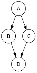
For example, when searching the directed graph below beginning at node A, the sequence of traversals is either A B D B A C A or A C D C A B A (choosing to first visit B or C from A is up to the algorithm). Note that repeat visits in the form of backtracking to a node, to check if it has still unvisited neighbors, are included here (even if it is found to have none). Thus the possible preorderings are A B D C and A C D B, while the possible postorderings are D B C A and D C B A, and the possible reverse postorderings are A C B D and A B C D.

Reverse postordering produces a topological sorting of any directed acyclic graph. This ordering is also useful in control-flow analysis as it often represents a natural linearization of the control flows. The graph above might represent the flow of control in the code fragment below, and it is natural to consider this code in the order A B C D or A C B D but not natural to use the order A B D C or A C D B.

if (A) then {     B } else {     C } D

Pseudocode

Input: Output: A recursive implementation of DFS: ^[5]

procedure DFS(G, v) is     label v as discovered     for all directed edges from v to w that areinG.adjacentEdges(v) doif vertex w is not labeled as discovered then             recursively call DFS(G, w)

A non-recursive implementation of DFS with worst-case space complexity ${\displaystyle O(|E|)}$, with the possibility of duplicate vertices on the stack: ^[6]

procedure DFS_iterative(G, v) is     let S be a stack     S.push(v)     whileS is not empty dov = S.pop()         ifv is not labeled as discovered then             label v as discovered             for all edges from v to winG.adjacentEdges(v) doS.push(w)

The example graph, copied from above

These two variations of DFS visit the neighbors of each vertex in the opposite order from each other: the first neighbor of v visited by the recursive variation is the first one in the list of adjacent edges, while in the iterative variation the first visited neighbor is the last one in the list of adjacent edges. The recursive implementation will visit the nodes from the example graph in the following order: A, B, D, F, E, C, G. The non-recursive implementation will visit the nodes as: A, E, F, B, D, C, G.

The non-recursive implementation is similar to breadth-first search but differs from it in two ways:

1. it uses a stack instead of a queue, and
2. it delays checking whether a vertex has been discovered until the vertex is popped from the stack rather than making this check before adding the vertex.

If G is a tree, replacing the queue of the breadth-first search algorithm with a stack will yield a depth-first search algorithm. For general graphs, replacing the stack of the iterative depth-first search implementation with a queue would also produce a breadth-first search algorithm, although a somewhat nonstandard one. ^[7]

Another possible implementation of iterative depth-first search uses a stack of iterators of the list of neighbors of a node, instead of a stack of nodes. This yields the same traversal as recursive DFS. ^[8]

procedure DFS_iterative(G, v) is     let S be a stack     label v as discovered     S.push(iterator of G.adjacentEdges(v))     whileS is not empty doifS.peek().hasNext() thenw = S.peek().next()             ifw is not labeled as discovered then                 label w as discovered                 S.push(iterator of G.adjacentEdges(w))         elseS.pop()

Applications

Randomized algorithm similar to depth-first search used in generating a maze.

Algorithms that use depth-first search as a building block include:

• Finding connected components.
• Topological sorting.
• Finding 2-(edge or vertex)-connected components.
• Finding 3-(edge or vertex)-connected components.
• Finding the bridges of a graph.
• Generating words in order to plot the limit set of a group.
• Finding strongly connected components.
• Determining whether a species is closer to one species or another in a phylogenetic tree.
• Planarity testing. ^{[9] [10]}
• Solving puzzles with only one solution, such as mazes. (DFS can be adapted to find all solutions to a maze by only including nodes on the current path in the visited set.)
• Maze generation may use a randomized DFS.
• Finding biconnectivity in graphs.
• Succession to the throne shared by the Commonwealth realms. ^[11]

Complexity

The computational complexity of DFS was investigated by John Reif. More precisely, given a graph ${\displaystyle G}$, let ${\displaystyle O=(v_{1},\dots ,v_{n})}$ be the ordering computed by the standard recursive DFS algorithm. This ordering is called the lexicographic depth-first search ordering. John Reif considered the complexity of computing the lexicographic depth-first search ordering, given a graph and a source. A decision version of the problem (testing whether some vertex u occurs before some vertex v in this order) is P-complete, ^[12] meaning that it is "a nightmare for parallel processing". ^{[13] : 189}

A depth-first search ordering (not necessarily the lexicographic one), can be computed by a randomized parallel algorithm in the complexity class RNC. ^[14] As of 1997, it remained unknown whether a depth-first traversal could be constructed by a deterministic parallel algorithm, in the complexity class NC. ^[15]

See also

• Tree traversal (for details about pre-order, in-order and post-order depth-first traversal)
• Breadth-first search
• Iterative deepening depth-first search
• Search game

Notes

1. Charles Pierre Trémaux (1859–1882) École polytechnique of Paris (X:1876), French engineer of the telegraph
   in Public conference, December 2, 2010 – by professor Jean Pelletier-Thibert in Académie de Macon (Burgundy – France) – (Abstract published in the Annals academic, March 2011 – ISSN   0980-6032)
2. Even, Shimon (2011), Graph Algorithms (2nd ed.), Cambridge University Press, pp. 46–48, ISBN   978-0-521-73653-4 .
3. Sedgewick, Robert (2002), Algorithms in C++: Graph Algorithms (3rd ed.), Pearson Education, ISBN   978-0-201-36118-6 .
4. Cormen, Thomas H., Charles E. Leiserson, and Ronald L. Rivest. p.606
5. Goodrich and Tamassia; Cormen, Leiserson, Rivest, and Stein
6. Page 93, Algorithm Design, Kleinberg and Tardos
7. "Stack-based graph traversal ≠ depth first search". 11011110.github.io. Retrieved 2020-06-10.
8. Sedgewick, Robert (2010). Algorithms in Java. Addison-Wesley. ISBN   978-0-201-36121-6. OCLC   837386973.
9. Hopcroft, John; Tarjan, Robert E. (1974), "Efficient planarity testing" (PDF), Journal of the Association for Computing Machinery , 21 (4): 549–568, doi:10.1145/321850.321852, hdl: 1813/6011 , S2CID   6279825 .
10. de Fraysseix, H.; Ossona de Mendez, P.; Rosenstiehl, P. (2006), "Trémaux Trees and Planarity", International Journal of Foundations of Computer Science, 17 (5): 1017–1030, arXiv: math/0610935 , Bibcode:2006math.....10935D, doi:10.1142/S0129054106004248, S2CID   40107560 .
11. Baccelli, Francois; Haji-Mirsadeghi, Mir-Omid; Khezeli, Ali (2018), "Eternal family trees and dynamics on unimodular random graphs", in Sobieczky, Florian (ed.), Unimodularity in Randomly Generated Graphs: AMS Special Session, October 8–9, 2016, Denver, Colorado, Contemporary Mathematics, vol. 719, Providence, Rhode Island: American Mathematical Society, pp. 85–127, arXiv: 1608.05940 , doi:10.1090/conm/719/14471, MR   3880014, S2CID   119173820 ; see Example 3.7, p. 93
12. Reif, John H. (1985). "Depth-first search is inherently sequential". Information Processing Letters. 20 (5): 229–234. doi:10.1016/0020-0190(85)90024-9.
13. Mehlhorn, Kurt; Sanders, Peter (2008). Algorithms and Data Structures: The Basic Toolbox (PDF). Springer. Archived (PDF) from the original on 2015-09-08.
14. Aggarwal, A.; Anderson, R. J. (1988), "A random NC algorithm for depth first search", Combinatorica , 8 (1): 1–12, doi:10.1007/BF02122548, MR   0951989, S2CID   29440871 .
15. Karger, David R.; Motwani, Rajeev (1997), "An NC algorithm for minimum cuts", SIAM Journal on Computing , 26 (1): 255–272, CiteSeerX   10.1.1.33.1701 , doi:10.1137/S0097539794273083, MR   1431256 .

References

• Thomas H. Cormen, Charles E. Leiserson, Ronald L. Rivest, and Clifford Stein. Introduction to Algorithms , Second Edition. MIT Press and McGraw-Hill, 2001. ISBN   0-262-03293-7. Section 22.3: Depth-first search, pp. 540–549.
• Goodrich, Michael T.; Tamassia, Roberto (2001), Algorithm Design: Foundations, Analysis, and Internet Examples, Wiley, ISBN   0-471-38365-1
• Kleinberg, Jon; Tardos, Éva (2006), Algorithm Design, Addison Wesley, pp. 92–94
• Knuth, Donald E. (1997), The Art of Computer Programming Vol 1. 3rd ed, Boston: Addison-Wesley, ISBN   0-201-89683-4, OCLC   155842391, archived from the original on 2008-09-04, retrieved 2008-02-12

External links

• Open Data Structures - Section 12.3.2 - Depth-First-Search, Pat Morin
• C++ Boost Graph Library: Depth-First Search
• Depth-First Search Animation (for a directed graph)
• Depth First and Breadth First Search: Explanation and Code
• QuickGraph ^{[ permanent dead link ]}, depth first search example for .Net
• Depth-first search algorithm illustrated explanation (Java and C++ implementations)
• YAGSBPL – A template-based C++ library for graph search and planning