Relationship between drag on an aircraft and other variables
The drag curve or drag polar is the relationship between the drag on an aircraft and other variables, such as lift, the coefficient of lift, angle-of-attack or speed. It may be described by an equation or displayed as a graph (sometimes called a "polar plot").[1] Drag may be expressed as actual drag or the coefficient of drag.
Drag curves are closely related to other curves which do not show drag, such as the power required/speed curve, or the sink rate/speed curve.
The drag curve
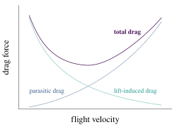
Drag and lift coefficients for the NACA 633618 airfoil. Full curves are lift, dashed drag; red curves have Re = 3·10 , blue 9·10 .Coefficients of lift and drag against angle of attack.Curve showing induced drag, parasitic drag and total drag as a function of airspeed.Drag curve for the NACA 633618 airfoil, colour-coded as opposite plot.
The lift and the drag forces, L and D, are scaled by the same factor to get CL and CD, so L/D = CL/CD. L and D are at right angles, with D parallel to the free stream velocity (the relative velocity of the surrounding distant air), so the resultant force R lies at the same angle to D as the line from the origin of the graph to the corresponding CL, CD point does to the CD axis.
If an aerodynamic surface is held at a fixed angle of attack in a wind tunnel, and the magnitude and direction of the resulting force are measured, they can be plotted using polar coordinates. When this measurement is repeated at different angles of attack the drag curve is obtained. Lift and drag data was gathered in this way in the 1880s by Otto Lilienthal and around 1910 by Gustav Eiffel, though not presented in terms of the more recent coefficients. Eiffel was the first to use the name "drag polar",[4] however drag curves are rarely plotted today using polar coordinates.
Depending on the aircraft type, it may be necessary to plot drag curves at different Reynolds and Mach numbers. The design of a fighter will require drag curves for different Mach numbers, whereas gliders, which spend their time either flying slowly in thermals or rapidly between them, may require curves at different Reynolds numbers but are unaffected by compressibility effects. During the evolution of the design the drag curve will be refined. A particular aircraft may have different curves even at the same Re and M values, depending for example on whether undercarriage and flaps are deployed.[2]
Drag curve for light aircraft. CD0= 0.017, K = 0.075 and CL0 = 0.1. The tangent gives the maximum L/D point.
The accompanying diagram shows CL against CD for a typical light aircraft. The minimum CD point is at the left-most point on the plot. One component of drag is induced drag (an inevitable side-effect of producing lift, which can be reduced by increasing the indicated airspeed). This is proportional to CL2. The other drag mechanisms, parasitic and wave drag, have both constant components, totalling CD0, and lift-dependent contributions that increase in proportion to CL2. In total, then
CD = CD0 + K.(CL - CL0)2.
The effect of CL0 is to shift the curve up the graph; physically this is caused by some vertical asymmetry, such as a cambered wing or a finite angle of incidence, which ensures the minimum drag attitude produces lift and increases the maximum lift-to-drag ratio.[2][5]
Power required curves
One example of the way the curve is used in the design process is the calculation of the power required (PR) curve, which plots the power needed for steady, level flight over the operating speed range. The forces involved are obtained from the coefficients by multiplication with (ρ/2).S V2, where ρ is the density of the atmosphere at the flight altitude, S is the wing area and V is the speed. In level flight, lift equals weight W and thrust equals drag, so
PR curve for the light aircraft with the drag curve above and weighing 2000 kg, with a wing area of 15 m² and a propeller efficiency of 0.8.
W = (ρ/2).S.V2.CL and
PR = (ρ/2η).S.V3.CD.
The extra factor of V/η, with η the propeller efficiency, in the second equation enters because PR= (required thrust)×V/η. Power rather than thrust is appropriate for a propeller driven aircraft, since it is roughly independent of speed; jet engines produce constant thrust. Since the weight is constant, the first of these equations determines how CL falls with increasing speed. Putting these CL values into the second equation with CD from the drag curve produces the power curve. The low speed region shows a fall in lift induced drag, through a minimum followed by an increase in profile drag at higher speeds. The minimum power required, at a speed of 195km/h (121mph) is about 86kW (115hp); 135kW (181hp) is required for a maximum speed of 300km/h (186mph). Flight at the power minimum will provide maximum endurance; the speed for greatest range is where the tangent to the power curve passes through the origin, about 240km/h (150mph).[6])
If an analytical expression for the curve is available, useful relationships can be developed by differentiation. For example the form above, simplified slightly by putting CL0 = 0, has a maximum CL/CD at CL2 = CD0/K. For a propeller aircraft this is the maximum endurance condition and gives a speed of 185km/h (115mph). The corresponding maximum range condition is the maximum of CL3/2/CD, at CL2 = 3.CD0/K, and so the optimum speed is 244km/h (152mph). The effects of the approximation CL0 = 0 are less than 5%; of course, with a finite CL0 = 0.1, the analytic and graphical methods give the same results.[6]
The low speed region of flight is known as the "back of the power curve" or "behind the power curve"[7][8] (sometimes "back of the drag curve") where more thrust is required to sustain flight at lower speeds. It is an inefficient region of flight because a decrease in speed requires increased thrust and a resultant increase in fuel consumption. It is regarded as a "speed unstable" region of flight, because unlike normal circumstances, a decrease in airspeed due to a nose-up pitch control input will not correct itself if the controls are returned to their previous position. Instead, airspeed will remain low and drag will progressively accumulate as airspeed and altitude continue to decay, and this condition will persist until thrust is increased, angle of attack is reduced (which will also shed altitude), or drag is otherwise reduced (such as by retracting the landing gear). Sustained flight behind the power curve requires alert piloting because inadequate thrust will cause a steady decrease in airspeed and a corresponding steady increase in descent rate, which may go unnoticed, and can be difficult to correct close to the ground. A not-infrequent result is the aircraft "mushing" and crashing short of the intended landing site because the pilot did not decrease angle of attack or increase thrust in time, or because adequate thrust is not available; the latter is a particular hazard during a forced landing after an engine failure.[8][9]
Failure to control airspeed and descent rate while flying behind the power curve has been implicated in a number of prominent aviation accidents, such as Asiana Airlines Flight 214.[9]
Rate of climb
For an aircraft to climb at an angle θ and at speed V its engine must be developing more power P in excess of power required PR to balance the drag experienced at that speed in level flight and shown on the power required plot. In level flight PR/V = D but in the climb there is the additional weight component to include, that is
P/V = D + W.sin θ = PR/V + W.sin θ.
Hence the climb rate RC = V.sin θ = (P - PR)/W.[10] Supposing the 135kW engine required for a maximum speed at 300km/h is fitted, the maximum excess power is 135 - 87 = 48Kw at the minimum of PR and the rate of climb 2.4m/s.
Fuel efficiency
For propeller aircraft (including turboprops), maximum range and therefore maximum fuel efficiency is achieved by flying at the speed for maximum lift-to-drag ratio. This is the speed which covers the greatest distance for a given amount of fuel. Maximum endurance (time in the air) is achieved at a lower speed, when drag is minimised.
For jet aircraft, maximum endurance occurs when the lift-to-drag ratio is maximised. Maximum range occurs at a higher speed. This is because jet engines are thrust-producing, not power-producing. Turboprop aircraft do produce some thrust through the turbine exhaust gases, however most of their output is as power through the propeller.
"Long-range cruise" speed (LRC) is typically chosen to give 1% less fuel efficiency than maximum range speed, because this results in a 3-5% increase in speed. However, fuel is not the only marginal cost in airline operations, so the speed for most economical operation (ECON) is chosen based on the cost index (CI), which is the ratio of time cost to fuel cost.[11]
Gliders
The same aircraft, without power. The tangent defines the minimum glide angle, for maximum range. The peak of the curve indicates the minimum sink rate, for maximum endurance (time in the air).
Without power, a gliding aircraft has only gravity to propel it. At a glide angle of , the weight has two components, at right angles to the flight line and parallel to it. These are balanced by the force and lift components respectively, so
and
Dividing one equation by the other shows that the glide angle is given by . The performance characteristics of most interest in unpowered flight are the speed across the ground, say, and the sink speed ; these are displayed by plotting against . Such plots are generally termed polars, and to produce them the glide angle as a function of is required.[12]
One way of finding solutions to the two force equations is to square them both then add together; this shows the possible , values lie on a circle of radius . When this is plotted on the drag polar, the intersection of the two curves locates the solution and its value read off. Alternatively, bearing in mind that glides are usually shallow, the approximation , good for less than 10°, can be used in the lift equation and the value of for a chosen calculated, finding from the drag polar and then calculating .[12]
The example polar here shows the gliding performance of the aircraft analysed above, assuming its drag polar is not much altered by the stationary propeller. A straight line from the origin to some point on the curve has a gradient equal to the glide angle at that speed, so the corresponding tangent shows the best glide angle . This is not the lowest rate of sink but provides the greatest range, requiring a speed of 240km/h (149mph); the minimum sink rate of about 3.5m/s is at 180km/h (112mph), speeds seen in the previous, powered plots.[12]
Sink rate
As airspeed increases, total drag decreases then increases.Polar curve for a glider, showing glide angle for minimum sink rate. The origin of the graph is where the airspeed axis crosses the sink rate axis at zero airspeed and zero sink rate. The horizontal line is tangent to the top of the polar curve. That tangent point indicates the minimum sink airspeed (vertical line). The sink rate increases to the left or right of this point, corresponding to a lower or higher airspeed. This minimum sink airspeed has the lowest possible rate of sink, and allows the longest possible glide time before landing.Polar curve for a glider, showing glide angle for the best glide speed (best L/D). It is the flattest possible glide angle through calm air, which will maximize the distance flown. This airspeed (vertical line) corresponds to the tangent point of a line starting from the origin of the graph. A glider flying faster or slower than this airspeed will cover less distance before landing.
A graph showing the sink rate of an aircraft (typically a glider) against its airspeed is known as a polar curve.[14] Polar curves are used to compute the glider's minimum sink speed, best lift over drag (L/D), and speed to fly.[13]
The polar curve of a glider is derived from theoretical calculations, or by measuring the rate of sink at various airspeeds. These data points are then connected by a line to form the curve. Each type of glider has a unique polar curve, and individual gliders vary somewhat depending on the smoothness of the wing, control surface drag, or the presence of bugs, dirt, and rain on the wing. Different glider configurations will have different polar curves, for example, solo versus dual flight, with and without water ballast, different flap settings, or with and without wing-tip extensions.[14]
Knowing the best speed to fly is important in exploiting the performance of a glider. Two of the key measures of a glider’s performance are its minimum sink rate and its best glide ratio, also known as the best "glide angle". These occur at different speeds. Knowing these speeds is important for efficient cross-country flying. In still air the polar curve shows that flying at the minimum sink speed enables the pilot to stay airborne for as long as possible and to climb as quickly as possible, but at this speed the glider will not travel as far as if it flew at the speed for the best glide.
Effect of wind, lift/sink and weight on best glide speed
The best speed to fly in a head wind is determined from the graph by shifting the origin to the right along the horizontal axis by the speed of the headwind, and drawing a new tangent line. This new airspeed will be faster as the headwind increases, but will result in the greatest distance covered. A general rule of thumb is to add half the headwind component to the best L/D for the maximum distance. For a tailwind, the origin is shifted to the left by the speed of the tailwind, and drawing a new tangent line. The tailwind speed to fly will lie between minimum sink and best L/D.[14]
In subsiding air, the polar curve is shifted lower according the airmass sink rate, and a new tangent line drawn. This will show the need to fly faster in subsiding air, which gives the subsiding air less time to lower the glider's altitude. Correspondingly, the polar curve is displaced upwards according to the lift rate, and a new tangent line drawn.[13]
Increased weight does not affect the maximum range of a gliding aircraft. Glide angle is only determined by the lift/drag ratio. Increased weight will require an increased airspeed to maintain the optimum glide angle, so a heavier gliding aircraft will have reduced endurance, because it is descending along the optimum glide path at a faster rate.[15]
For racing, glider pilots will often use water ballast to increase the weight of their glider. This increases the optimum speed, at a cost of low speed performance and a reduced climb rate in thermals.[16] Ballast can also be used to adjust the centre of gravity of the glider, which can improve performance.
Glider Performance Airspeeds – an animated explanation of the basic polar curve, with modifications for sinking or rising air and for head- or tailwinds.
References
↑ Shames, Irving H. (1962). Mechanics of Fluids. McGraw-Hill. p.364. LCCN61-18731. Retrieved 8 November 2012. Another useful curve that is commonly used in reporting wind-tunnel data is the CL vs CD curve, which is sometimes called the polar plot.
1 2 3 Anderson, John D. Jnr. (1999). Aircraft Performance and Design. Cambridge: WCB/McGraw-Hill. ISBN0-07-116010-8.
↑ Abbott, Ira H.; von Doenhoff, Albert E. (1958). Theory of wing sections. New York: Dover Publications. pp.57–70, 129–142. ISBN0-486-60586-8.{{cite book}}: ISBN / Date incompatibility (help)
This page is based on this Wikipedia article Text is available under the CC BY-SA 4.0 license; additional terms may apply. Images, videos and audio are available under their respective licenses.