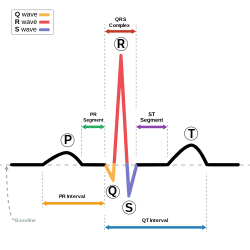
Last updated Simulation of a realistic heart beat.Schematic diagram of normal sinus rhythm for a human heart as seen on ECG.
The forward problem of electrocardiology is a computational and mathematical approach to study the electrical activity of the heart through the body surface.[1] The principal aim of this study is to computationally reproduce an electrocardiogram (ECG), which has important clinical relevance to define cardiac pathologies such as ischemia and infarction, or to test pharmaceutical intervention. Given their important functionalities and the relative small invasiveness, the electrocardiography techniques are used quite often as clinical diagnostic tests. Thus, it is natural to proceed to computationally reproduce an ECG, which means to mathematically model the cardiac behaviour inside the body.[1]
Thus, to obtain an ECG, a mathematical electrical cardiac model must be considered, coupled with a diffusive model in a passive conductor that describes the electrical propagation inside the torso.[1]
The coupled model is usually a three-dimensional model expressed in terms of partial differential equations. Such model is typically solved by means of finite element method for the solution's space evolution and semi-implicit numerical schemes involving finite differences for the solution's time evolution. However, the computational costs of such techniques, especially with three dimensional simulations, are quite high. Thus, simplified models are often considered, solving for example the heart electrical activity independently from the problem on the torso. To provide realistic results, three dimensional anatomically realistic models of the heart and the torso must be used.[1]
The electrical activity of the heart is caused by the flow of ions across the cell membrane, between the intracellular and extracellular spaces, which determines a wave of excitation along the heart muscle that coordinates the cardiac contraction and, thus, the pumping action of the heart that enables it to push blood through the circulatory system. The modeling of cardiac electrical activity is thus related to the modelling of the flow of ions on a microscopic level, and on the propagation of the excitation wave along the muscle fibers on a macroscopic level.[1][4]
Between the mathematical model on the macroscopic level, Willem Einthoven and Augustus Waller defined the ECG through the conceptual model of a dipole rotating around a fixed point, whose projection on the lead axis determined the lead recordings. Then, a two-dimensional reconstruction of the heart activity in the frontal plane was possible using the Einthoven's limbs leads I, II and III as theoretical basis.[5] Later on, the rotating cardiac dipole was considered inadequate and was substituted by multipolar sources moving inside a bounded torso domain. The main shortcoming of the methods used to quantify these sources is their lack of details, which are however very relevant to realistically simulate cardiac phenomena.[4]
On the other hand, microscopic models try to represent the behaviour of single cells and to connect them considering their electrical properties.[6][7][8] These models present some challenges related to the different scales that need to be captured, in particular considering that, especially for large scale phenomena such as re-entry or body surface potential, the collective behaviour of the cells is more important than that of every single cell.[4]
The third option to model the electrical activity of the heart is to consider a so-called "middle-out approach", where the model incorporates both lower and higher level of details. This option considers the behaviour of a block of cells, called a continuum cell, thus avoiding scale and detail problems. The model obtained is called bidomain model, which is often replaced by its simplification, the monodomain model.[4]
Stylized representation of a human torso that describes the domain and the notation considered for the forward problem of electrocardiography. Two separated areas and their boundary are considered, which represent the heart and human torso around it.
The basic assumption of the bidomain model is that the heart tissue can be divided in two ohmic conducting continuous media, connected but separated through the cell membrane. This media are called intracellular and extracellular regions, the former representing the cellular tissues, and the latter representing the space between cells.[2][1]
The standard formulation of the bidomain model, including a dynamical model for the ionic current, is the following[2] where and are the transmembrane and extracellular potentials respectively, is the ionic current, which depends also from a so-called gating variable (accounting for cellular-level ionic behavior), and is an external current applied to the domain. Moreover, and are the intracellular and extracellular conductivity tensors, is the surface to volume ratio of the cell membrane and is the membrane capacitance per unit area. Here the domain represents the heart muscle.[2]
The boundary conditions for this version of the bidomain model are obtained through the assumption that there is no flow of intracellular potential outside of the heart, which means that where denotes the boundary of the heart domain and is the outward unit normal to .[2]
The monodomain model is a simplification of the bidomain model that, in spite of some unphysiological assumptions, is able to represent realistic electrophysiological phenomena at least for what concerns the transmembrane potential .[2][1]
The standard formulation is the following partial differential equation, whose only unknown is the transmembrane potential: where is a parameter that relates the intracellular and extracellular conductivity tensors.[2]
In the forward problem of electrocardiography, the torso is seen as a passive conductor and its model can be derived starting from the Maxwell's equations under quasi-static assumption.[1][2]
The standard formulation consists of a partial differential equation with one unknown scalar field, the torso potential . Basically, the torso model is the following generalized Laplace equation where is the conductivity tensor and is the domain surrounding the heart, i.e. the human torso.[2]
Derivation
As for the bidomain model, the torso model can be derived from the Maxwell's equations and the continuity equation after some assumptions. First of all, since the electrical and magnetic activity inside the body is generated at low level, a quasi-static assumption can be considered. Thus, the body can be viewed as a passive conductor, which means that its capacitive, inductive and propagative effect can be ignored.[1]
Under quasi-static assumption, the Maxwell's equations are[1] and the continuity equation is[1]
Since its curl is zero, the electrical field can be represented by the gradient of a scalar potential field, the torso potential
1
where the negative sign means that the current flows from higher to lower potential regions.[1]
Then, the total current density can be expressed in terms of the conduction current and other different applied currents so that, from continuity equation,[1]
Finally, since aside from the heart there is no current source inside the torso, the current per unit volume can be set to zero, giving the generalized Laplace equation, which represents the standard formulation of the diffusive problem inside the torso[1]
Boundary condition
The boundary conditions accounts for the properties of the media surrounding the torso, i.e. of the air around the body. Generally, air has null conductivity which means that the current cannot flow outside the torso. This is translated in the following equation[1]
where is the unit outward normal to the torso and is the torso boundary, which means the torso surface.[1][2]
Torso conductivity
Usually, the torso is considered to have isotropic conductivity, which means that the current flows in the same way in all directions. However, the torso is not an empty or homogeneous envelope, but contains different organs characterized by different conductivity coefficients, which can be experimentally obtained. A simple example of conductivity parameters in a torso that considers the bones and the lungs is reported in the following table.[2]
The coupling between the electrical activity model and the torso model is achieved by means of suitable boundary conditions at the epicardium, i.e. at the interface surface between the heart and the torso.[1][2]
The heart-torso model can be fully coupled, if a perfect electrical transmission between the two domains is considered, or can be uncoupled, if the heart electrical model and the torso model are solved separately with a limited or imperfect exchange of information between them.[2]
Fully coupled heart-torso models
The complete coupling between the heart and the torso is obtained imposing a perfect electrical transmission condition between the heart and the torso. This is done considering the following two equations, that establish a relationship between the extracellular potential and the torso potential[2] This equations ensure the continuity of both the potential and the current across the epicardium.[2]
Using these boundary conditions, it is possible to obtain two different fully coupled heart-torso models, considering either the bidomain or the monodomain model for the heart electrical activity. From the numerical viewpoint, the two models are computationally very expensive and have similar computational costs.[2]
Alternative boundary conditions
Boundary conditions that represent a perfect electrical coupling between the heart and the torso are the most used and the classical ones. However, between the heart and the torso there is the pericardium, a sac with a double wall that contains a serous fluid which has a specific effect on the electrical transmission. Considering the capacitance and the resistive effect that the pericardium has, alternative boundary conditions that take into account this effect can be formulated as follows[10]
Formulation with the bidomain model
The fully coupled heart-torso model, considering the bidomain model for the heart electrical activity, in its complete form is[2] where the first four equations are the partial differential equations representing the bidomain model, the ionic model and the torso model, while the remaining ones represent the boundary conditions for the bidomain and torso models and the coupling conditions between them.[2]
Formulation with the monodomain model
The fully coupled heart-torso model considering the monodomain model for the electrical activity of the heart is more complicated that the bidomain problem. Indeed, the coupling conditions relate the torso potential with the extracellular potential, which is not computed by the monodomain model. Thus, it is necessary to use also the second equation of the bidomain model (under the same assumptions under which the monodomain model is derived), yielding:[2]
This way, the coupling conditions do not need to be changed, and the complete heart-torso model is composed of two different blocks:[2]
First the monodomain model with its usual boundary condition must be solved:
Then, the coupled model that includes the computation of the extracellular potential, the torso model and the coupling conditions must be solved:
Uncoupled heart-torso models
The fully coupled heart-torso models are very detailed models but they are also computationally expensive to solve.[2] A possible simplification is provided by the so-called uncoupled assumption in which the heart is considered completely electrically isolated from the heart.[2] Mathematically, this is done imposing that the current cannot flow across the epicardium, from the heart to the torso, namely[2]
Applying this equation to the boundary conditions of the fully coupled models, it is possible to obtained two uncoupled heart-torso models, in which the electrical models can be solved separately from the torso model reducing the computational costs.[2]
Uncoupled heart-torso model with the bidomain model
The uncoupled version of the fully coupled heart-torso model that uses the bidomain to represent the electrical activity of the heart is composed of two separated parts:[2]
The torso diffusive model in its standard formulation, with the potential continuity condition
Uncoupled heart-torso model with the modomain model
As in the case of the fully coupled heart-torso model which uses the monodomain model, also in the corresponding uncoupled model extracellular potential needs to be computed. In this case, three different and independent problems must be solved:[2]
The monodomain model with its usual boundary condition:
The problem to compute the extracellular potential with a boundary condition on the epicardium prescribing no intracellular current flow:
The torso diffusive model with the potential continuity boundary condition at the epicardium:
Solving the fully coupled or the uncoupled heart-torso models allows to obtain the electrical potential generated by the heart in every point of the human torso, and in particular on the whole surface of the torso. Defining the electrodes positions on the torso, it is possible to find the time evolution of the potential on such points. Then, the electrocardiograms can be computed, for example according to the 12 standard leads, considering the following formulas[2] where and are the standard locations of the electrodes.[2]
Numerical methods
The heart-torso models are expressed in terms of partial differential equations whose unknowns are function of both space and time. They are in turn coupled with an ionic model which is usually expressed in terms of a system of ordinary differential equations. A variety of numerical schemes can be used for the solution of those problems. Usually, the finite element method is applied for the space discretization and semi-implicit finite-difference schemes are used for the time discretization.[1][2]
Uncoupled heart-torso model are the simplest to treat numerically because the heart electrical model can be solved separately from the torso one, so that classic numerical methods to solve each of them can be applied. This means that the bidomain and monodomain models can be solved for example with a backward differentiation formula for the time discretization, while the problems to compute the extracellular potential and torso potential can be easily solved by applying only the finite element method because they are time independent.[1][2]
The fully coupled heart-torso models, instead, are more complex and need more sophisticated numerical models. For example, the fully heart-torso model that uses the bidomain model for the electrical simulation of the cardiac behaviour can be solved considering domain decomposition techniques, such as a Dirichlet-Neumann domain decomposition.[2][11]
Geometric torso model
Three-dimensional torso model including the most organs.
To simulate and electrocardiogram using the fully coupled or uncoupled models, a three-dimensional reconstruction of the human torso is needed. Today, diagnostic imaging techniques such as MRI and CT can provide a sufficiently accurate images that allow to reconstruct in detail anatomical human parts and, thus, obtain a suitable torso geometry. For example, the Visible Human Data[13] is a useful dataset to create a three-dimensional torso model detailed with internal organs including the skeletal structure and muscles.[1]
Dynamical model for the electrocardiogram
Even if the results are quite detailed, solving a three-dimensional model is usually quite expensive. A possible simplification is a dynamical model based on three coupled ordinary differential equations.[3]
The quasi-periodicity of the heart beat is reproduced by a three-dimensional trajectory around an attracting limit cycle in the plane. The principal peaks of the ECG, which are the P,Q,R,S and T, are described at fixed angles , which give the following three ODEs[3]
with , ,
The equations can be easily solved with classical numerical algorithms like Runge-Kutta methods for ODEs.[3]
1 2 3 4 Lines, G.T.; Buist, M.L.; Grottum, P.; Pullan, A.J.; Sundnes, J.; Tveito, A. (1 July 2002). "Mathematical models and numerical methods for the forward problem in cardiac electrophysiology". Computing and Visualization in Science. 5 (4): 215–239. doi:10.1007/s00791-003-0101-4. S2CID123211416.
↑ Henriquez, C.S.; Plonsey, R. (1987). "Effect of resistive discontinuities on waveshape and velocity in a single cardiac fibre". Med. Biol. Eng. Comput. 25 (4): 428–438. doi:10.1007/BF02443364. PMID3450994. S2CID3038844.
↑ Keener, James; Sneyd, James (2009). Mathematical physiology 2009: systems physiology ii (2nd reviseditioned.). Springer. ISBN978-1-4939-3709-7.
↑ Boulakia, Muriel; Fernández, Miguel A.; Gerbeau, Jean-Frédéric; Zemzemi, Nejib (2007). "Towards the Numerical Simulation of Electrocardiograms". Functional Imaging and Modeling of the Heart. Lecture Notes in Computer Science. Vol.4466. Springer. pp.240–249. doi:10.1007/978-3-540-72907-5_25. ISBN978-3-540-72906-8.
This page is based on this Wikipedia article Text is available under the CC BY-SA 4.0 license; additional terms may apply. Images, videos and audio are available under their respective licenses.