Kernel density estimation

Kernel density estimation of 100 normally distributed random numbers using different smoothing bandwidths.

In statistics, kernel density estimation (KDE) is the application of kernel smoothing for probability density estimation, i.e., a non-parametric method to estimate the probability density function of a random variable based on kernels as weights. KDE answers a fundamental data smoothing problem where inferences about the population are made based on a finite data sample. In some fields such as signal processing and econometrics it is also termed the Parzen–Rosenblatt window method, after Emanuel Parzen and Murray Rosenblatt, who are usually credited with independently creating it in its current form. ^{[1] [2]} One of the famous applications of kernel density estimation is in estimating the class-conditional marginal densities of data when using a naive Bayes classifier, ^{[3] [4]} which can improve its prediction accuracy. ^[3]

Definition

Let (x₁, x₂, ..., x_n) be independent and identically distributed samples drawn from some univariate distribution with an unknown density ƒ at any given point x. We are interested in estimating the shape of this function ƒ. Its kernel density estimator is

${\displaystyle {\widehat {f}}_{h}(x)={\frac {1}{n}}\sum _{i=1}^{n}K_{h}(x-x_{i})={\frac {1}{nh}}\sum _{i=1}^{n}K{\Big (}{\frac {x-x_{i}}{h}}{\Big )},}$

where K is the kernel — a non-negative function — and h > 0 is a smoothing parameter called the bandwidth. A kernel with subscript h is called the scaled kernel and defined as K_h(x) = ${\displaystyle {\tfrac {1}{h}}}$K(${\displaystyle {\tfrac {x}{h}}}$). Intuitively one wants to choose h as small as the data will allow; however, there is always a trade-off between the bias of the estimator and its variance. The choice of bandwidth is discussed in more detail below.

A range of kernel functions are commonly used: uniform, triangular, biweight, triweight, Epanechnikov, normal, and others. The Epanechnikov kernel is optimal in a mean square error sense, ^[5] though the loss of efficiency is small for the kernels listed previously. ^[6] Due to its convenient mathematical properties, the normal kernel is often used, which means K(x) = ϕ(x), where ϕ is the standard normal density function.

The construction of a kernel density estimate finds interpretations in fields outside of density estimation. ^[7] For example, in thermodynamics, this is equivalent to the amount of heat generated when heat kernels (the fundamental solution to the heat equation) are placed at each data point locations x_i. Similar methods are used to construct discrete Laplace operators on point clouds for manifold learning (e.g. diffusion map).

Example

Kernel density estimates are closely related to histograms, but can be endowed with properties such as smoothness or continuity by using a suitable kernel. The diagram below based on these 6 data points illustrates this relationship:

Sample	1	2	3	4	5	6
Value	−2.1	−1.3	−0.4	1.9	5.1	6.2

For the histogram, first, the horizontal axis is divided into sub-intervals or bins which cover the range of the data: In this case, six bins each of width 2. Whenever a data point falls inside this interval, a box of height 1/12 is placed there. If more than one data point falls inside the same bin, the boxes are stacked on top of each other.

For the kernel density estimate, normal kernels with a standard deviation of 1.5 (indicated by the red dashed lines) are placed on each of the data points x_i. The kernels are summed to make the kernel density estimate (solid blue curve). The smoothness of the kernel density estimate (compared to the discreteness of the histogram) illustrates how kernel density estimates converge faster to the true underlying density for continuous random variables. ^[8]

Comparison of the histogram (left) and kernel density estimate (right) constructed using the same data. The six individual kernels are the red dashed curves, the kernel density estimate the blue curves. The data points are the rug plot on the horizontal axis.

Bandwidth selection

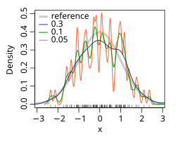
Kernel density estimate (KDE) with different bandwidths of a random sample of 100 points from a standard normal distribution. Grey: true density (standard normal). Red: KDE with h=0.05. Black: KDE with h=0.337. Green: KDE with h=2.

The bandwidth of the kernel is a free parameter which exhibits a strong influence on the resulting estimate. To illustrate its effect, we take a simulated random sample from the standard normal distribution (plotted at the blue spikes in the rug plot on the horizontal axis). The grey curve is the true density (a normal density with mean 0 and variance 1). In comparison, the red curve is undersmoothed since it contains too many spurious data artifacts arising from using a bandwidth h = 0.05, which is too small. The green curve is oversmoothed since using the bandwidth h = 2 obscures much of the underlying structure. The black curve with a bandwidth of h = 0.337 is considered to be optimally smoothed since its density estimate is close to the true density. An extreme situation is encountered in the limit ${\displaystyle h\to 0}$ (no smoothing), where the estimate is a sum of n delta functions centered at the coordinates of analyzed samples. In the other extreme limit ${\displaystyle h\to \infty }$ the estimate retains the shape of the used kernel, centered on the mean of the samples (completely smooth).

The most common optimality criterion used to select this parameter is the expected L₂ risk function, also termed the mean integrated squared error:

${\displaystyle \operatorname {MISE} (h)=\operatorname {E} \!\left[\,\int ({\hat {f}}_{h}(x)-f(x))^{2}\,dx\right]}$

Under weak assumptions on ƒ and K, (ƒ is the, generally unknown, real density function), ^{[1] [2]}

${\displaystyle \operatorname {MISE} (h)=\operatorname {AMISE} (h)+{\mathcal {o}}((nh)^{-1}+h^{4})}$

where o is the little o notation, and n the sample size (as above). The AMISE is the asymptotic MISE, i. e. the two leading terms,

${\displaystyle \operatorname {AMISE} (h)={\frac {R(K)}{nh}}+{\frac {1}{4}}m_{2}(K)^{2}h^{4}R(f'')}$

where ${\displaystyle R(g)=\int g(x)^{2}\,dx}$ for a function g, ${\displaystyle m_{2}(K)=\int x^{2}K(x)\,dx}$ and ${\displaystyle f''}$ is the second derivative of ${\displaystyle f}$ and ${\displaystyle K}$ is the kernel. The minimum of this AMISE is the solution to this differential equation

${\displaystyle {\frac {\partial }{\partial h}}\operatorname {AMISE} (h)=-{\frac {R(K)}{nh^{2}}}+m_{2}(K)^{2}h^{3}R(f'')=0}$

or

${\displaystyle h_{\operatorname {AMISE} }={\frac {R(K)^{1/5}}{m_{2}(K)^{2/5}R(f'')^{1/5}}}n^{-1/5}=Cn^{-1/5}}$

Neither the AMISE nor the h_AMISE formulas can be used directly since they involve the unknown density function ${\displaystyle f}$ or its second derivative ${\displaystyle f''}$. To overcome that difficulty, a variety of automatic, data-based methods have been developed to select the bandwidth. Several review studies have been undertaken to compare their efficacies, ^{[9] [10] [11] [12] [13] [14] [15]} with the general consensus that the plug-in selectors ^{[7] [16] [17]} and cross validation selectors ^{[18] [19] [20]} are the most useful over a wide range of data sets.

Substituting any bandwidth h which has the same asymptotic order n^−1/5 as h_AMISE into the AMISE gives that AMISE(h) = O(n^−4/5), where O is the big O notation. It can be shown that, under weak assumptions, there cannot exist a non-parametric estimator that converges at a faster rate than the kernel estimator. ^[21] Note that the n^−4/5 rate is slower than the typical n⁻¹ convergence rate of parametric methods.

If the bandwidth is not held fixed, but is varied depending upon the location of either the estimate (balloon estimator) or the samples (pointwise estimator), this produces a particularly powerful method termed adaptive or variable bandwidth kernel density estimation.

Bandwidth selection for kernel density estimation of heavy-tailed distributions is relatively difficult. ^[22]

A rule-of-thumb bandwidth estimator

If Gaussian basis functions are used to approximate univariate data, and the underlying density being estimated is Gaussian, the optimal choice for h (that is, the bandwidth that minimises the mean integrated squared error) is: ^[23]

${\displaystyle h=\left({\frac {4{\hat {\sigma }}^{5}}{3n}}\right)^{\frac {1}{5}}\approx 1.06\,{\hat {\sigma }}\,n^{-1/5},}$

An ${\displaystyle h}$ value is considered more robust when it improves the fit for long-tailed and skewed distributions or for bimodal mixture distributions. This is often done empirically by replacing the standard deviation ${\displaystyle {\hat {\sigma }}}$ by the parameter ${\displaystyle A}$ below:

${\displaystyle A=\min \left({\hat {\sigma }},{\frac {IQR}{1.34}}\right)}$ where IQR is the interquartile range.

Comparison between rule of thumb and solve-the-equation bandwidth.

Another modification that will improve the model is to reduce the factor from 1.06 to 0.9. Then the final formula would be:

${\displaystyle h=0.9\,\min \left({\hat {\sigma }},{\frac {IQR}{1.34}}\right)\,n^{-{\frac {1}{5}}}}$

where ${\displaystyle n}$ is the sample size.

This approximation is termed the normal distribution approximation, Gaussian approximation, or Silverman's rule of thumb. ^[23] While this rule of thumb is easy to compute, it should be used with caution as it can yield widely inaccurate estimates when the density is not close to being normal. For example, when estimating the bimodal Gaussian mixture model

${\displaystyle {\frac {1}{2{\sqrt {2\pi }}}}e^{-{\frac {1}{2}}(x-10)^{2}}+{\frac {1}{2{\sqrt {2\pi }}}}e^{-{\frac {1}{2}}(x+10)^{2}}}$

from a sample of 200 points, the figure on the right shows the true density and two kernel density estimates — one using the rule-of-thumb bandwidth, and the other using a solve-the-equation bandwidth. ^{[7] [17]} The estimate based on the rule-of-thumb bandwidth is significantly oversmoothed.

Relation to the characteristic function density estimator

Given the sample (x₁, x₂, ..., x_n), it is natural to estimate the characteristic function φ(t) = E[e^itX] as

${\displaystyle {\widehat {\varphi }}(t)={\frac {1}{n}}\sum _{j=1}^{n}e^{itx_{j}}}$

Knowing the characteristic function, it is possible to find the corresponding probability density function through the Fourier transform formula. One difficulty with applying this inversion formula is that it leads to a diverging integral, since the estimate ${\displaystyle \scriptstyle {\widehat {\varphi }}(t)}$ is unreliable for large t’s. To circumvent this problem, the estimator ${\displaystyle \scriptstyle {\widehat {\varphi }}(t)}$ is multiplied by a damping function ψ_h(t) = ψ(ht), which is equal to 1 at the origin and then falls to 0 at infinity. The “bandwidth parameter” h controls how fast we try to dampen the function ${\displaystyle \scriptstyle {\widehat {\varphi }}(t)}$. In particular when h is small, then ψ_h(t) will be approximately one for a large range of t’s, which means that ${\displaystyle \scriptstyle {\widehat {\varphi }}(t)}$ remains practically unaltered in the most important region of t’s.

The most common choice for function ψ is either the uniform function ψ(t) = 1{−1 ≤ t ≤ 1}, which effectively means truncating the interval of integration in the inversion formula to [−1/h, 1/h], or the Gaussian function ψ(t) = e^−πt2. Once the function ψ has been chosen, the inversion formula may be applied, and the density estimator will be

${\displaystyle {\begin{aligned}{\widehat {f}}(x)&={\frac {1}{2\pi }}\int _{-\infty }^{+\infty }{\widehat {\varphi }}(t)\psi _{h}(t)e^{-itx}\,dt={\frac {1}{2\pi }}\int _{-\infty }^{+\infty }{\frac {1}{n}}\sum _{j=1}^{n}e^{it(x_{j}-x)}\psi (ht)\,dt\\[5pt]&={\frac {1}{nh}}\sum _{j=1}^{n}{\frac {1}{2\pi }}\int _{-\infty }^{+\infty }e^{-i(ht){\frac {x-x_{j}}{h}}}\psi (ht)\,d(ht)={\frac {1}{nh}}\sum _{j=1}^{n}K{\Big (}{\frac {x-x_{j}}{h}}{\Big )},\end{aligned}}}$

where K is the Fourier transform of the damping function ψ. Thus the kernel density estimator coincides with the characteristic function density estimator.

Geometric and topological features

We can extend the definition of the (global) mode to a local sense and define the local modes:

${\displaystyle M=\{x:g(x)=0,\lambda _{1}(x)<0\}}$

Namely, ${\displaystyle M}$ is the collection of points for which the density function is locally maximized. A natural estimator of ${\displaystyle M}$ is a plug-in from KDE, ^{[24] [25]} where ${\displaystyle g(x)}$ and ${\displaystyle \lambda _{1}(x)}$ are KDE version of ${\displaystyle g(x)}$ and ${\displaystyle \lambda _{1}(x)}$. Under mild assumptions, ${\displaystyle M_{c}}$ is a consistent estimator of ${\displaystyle M}$. Note that one can use the mean shift algorithm ^{[26] [27] [28]} to compute the estimator ${\displaystyle M_{c}}$ numerically.

Statistical implementation

A non-exhaustive list of software implementations of kernel density estimators includes:

• In Analytica release 4.4, the Smoothing option for PDF results uses KDE, and from expressions it is available via the built-in Pdf function.
• In C/C++, FIGTree is a library that can be used to compute kernel density estimates using normal kernels. MATLAB interface available.
• In C++, libagf is a library for variable kernel density estimation.
• In C++, mlpack is a library that can compute KDE using many different kernels. It allows to set an error tolerance for faster computation. Python and R interfaces are available.
• in C# and F#, Math.NET Numerics is an open source library for numerical computation which includes kernel density estimation
• In CrimeStat, kernel density estimation is implemented using five different kernel functions – normal, uniform, quartic, negative exponential, and triangular. Both single- and dual-kernel density estimate routines are available. Kernel density estimation is also used in interpolating a Head Bang routine, in estimating a two-dimensional Journey-to-crime density function, and in estimating a three-dimensional Bayesian Journey-to-crime estimate.
• In ELKI, kernel density functions can be found in the package de.lmu.ifi.dbs.elki.math.statistics.kernelfunctions
• In ESRI products, kernel density mapping is managed out of the Spatial Analyst toolbox and uses the Quartic(biweight) kernel.
• In Excel, the Royal Society of Chemistry has created an add-in to run kernel density estimation based on their Analytical Methods Committee Technical Brief 4.
• In gnuplot, kernel density estimation is implemented by the smooth kdensity option, the datafile can contain a weight and bandwidth for each point, or the bandwidth can be set automatically ^[29] according to "Silverman's rule of thumb" (see above).
• In Haskell, kernel density is implemented in the statistics package.
• In IGOR Pro, kernel density estimation is implemented by the StatsKDE operation (added in Igor Pro 7.00). Bandwidth can be user specified or estimated by means of Silverman, Scott or Bowmann and Azzalini. Kernel types are: Epanechnikov, Bi-weight, Tri-weight, Triangular, Gaussian and Rectangular.
• In Java, the Weka machine learning package provides weka.estimators.KernelEstimator, among others.
• In JavaScript, the visualization package D3.js offers a KDE package in its science.stats package.
• In JMP, the Graph Builder platform utilizes kernel density estimation to provide contour plots and high density regions (HDRs) for bivariate densities, and violin plots and HDRs for univariate densities. Sliders allow the user to vary the bandwidth. Bivariate and univariate kernel density estimates are also provided by the Fit Y by X and Distribution platforms, respectively.
• In Julia, kernel density estimation is implemented in the KernelDensity.jl package.
• In KNIME, 1D and 2D Kernel Density distributions can be generated and plotted using nodes from the Vernalis community contribution, e.g. 1D Kernel Density Plot, among others. The underlying implementation is written in Java.
• In MATLAB, kernel density estimation is implemented through the ksdensity function (Statistics Toolbox). As of the 2018a release of MATLAB, both the bandwidth and kernel smoother can be specified, including other options such as specifying the range of the kernel density. ^[30] Alternatively, a free MATLAB software package which implements an automatic bandwidth selection method ^[7] is available from the MATLAB Central File Exchange for
  • 1-dimensional data
  • 2-dimensional data
  • n-dimensional data
    A free MATLAB toolbox with implementation of kernel regression, kernel density estimation, kernel estimation of hazard function and many others is available on these pages (this toolbox is a part of the book ^[31] ).
• In Mathematica, numeric kernel density estimation is implemented by the function SmoothKernelDistribution ^[32] and symbolic estimation is implemented using the function KernelMixtureDistribution ^[33] both of which provide data-driven bandwidths.
• In Minitab, the Royal Society of Chemistry has created a macro to run kernel density estimation based on their Analytical Methods Committee Technical Brief 4. ^[34]
• In the NAG Library, kernel density estimation is implemented via the g10ba routine (available in both the Fortran ^[35] and the C ^[36] versions of the Library).
• In Nuklei, C++ kernel density methods focus on data from the Special Euclidean group ${\displaystyle SE(3)}$.
• In Octave, kernel density estimation is implemented by the kernel_density option (econometrics package).
• In Origin, 2D kernel density plot can be made from its user interface, and two functions, Ksdensity for 1D and Ks2density for 2D can be used from its LabTalk, Python, or C code.
• In Perl, an implementation can be found in the Statistics-KernelEstimation module
• In PHP, an implementation can be found in the MathPHP library
• In Python, many implementations exist: pyqt_fit.kde Module in the PyQt-Fit package, SciPy (scipy.stats.gaussian_kde), Statsmodels (KDEUnivariate and KDEMultivariate), and scikit-learn (KernelDensity) (see comparison ^[37] ). KDEpy supports weighted data and its FFT implementation is orders of magnitude faster than the other implementations. The commonly used pandas library offers support for kde plotting through the plot method (df.plot(kind='kde') ). The getdist package for weighted and correlated MCMC samples supports optimized bandwidth, boundary correction and higher-order methods for 1D and 2D distributions. One newly used package for kernel density estimation is seaborn ( import seaborn as sns , sns.kdeplot() ). ^[38] A GPU implementation of KDE also exists. ^[39]
• In R, it is implemented through density in the base distribution, and bw.nrd0 function is used in stats package, this function uses the optimized formula in Silverman's book. bkde in the KernSmooth library, ParetoDensityEstimation in the DataVisualizations library (for pareto distribution density estimation), kde in the ks library, dkden and dbckden in the evmix library (latter for boundary corrected kernel density estimation for bounded support), npudens in the np library (numeric and categorical data), sm.density in the sm library. For an implementation of the kde.R function, which does not require installing any packages or libraries, see kde.R. The btb library, dedicated to urban analysis, implements kernel density estimation through kernel_smoothing.
• In SAS, proc kde can be used to estimate univariate and bivariate kernel densities.
• In Apache Spark, the KernelDensity() class ^[40]
• In Stata, it is implemented through kdensity; ^[41] for example histogram x, kdensity. Alternatively a free Stata module KDENS is available ^[42] allowing a user to estimate 1D or 2D density functions.
• In Swift, it is implemented through SwiftStats.KernelDensityEstimation in the open-source statistics library SwiftStats.

See also

• Kernel (statistics)
• Kernel smoothing
• Kernel regression
• Density estimation (with presentation of other examples)
• Mean-shift
• Scale space: The triplets {(x, h, KDE with bandwidth h evaluated at x: all x, h > 0} form a scale space representation of the data.
• Multivariate kernel density estimation
• Variable kernel density estimation
• Head/tail breaks

Further reading

• Härdle, Müller, Sperlich, Werwatz, Nonparametric and Semiparametric Methods, Springer-Verlag Berlin Heidelberg 2004, pp. 39–83

References

1. Rosenblatt, M. (1956). "Remarks on Some Nonparametric Estimates of a Density Function". The Annals of Mathematical Statistics. 27 (3): 832–837. doi: 10.1214/aoms/1177728190 .
2. Parzen, E. (1962). "On Estimation of a Probability Density Function and Mode". The Annals of Mathematical Statistics . 33 (3): 1065–1076. doi: 10.1214/aoms/1177704472 . JSTOR   2237880.
3. Piryonesi S. Madeh; El-Diraby Tamer E. (2020-06-01). "Role of Data Analytics in Infrastructure Asset Management: Overcoming Data Size and Quality Problems". Journal of Transportation Engineering, Part B: Pavements. 146 (2): 04020022. doi:10.1061/JPEODX.0000175. S2CID   216485629.
4. Hastie, Trevor; Tibshirani, Robert; Friedman, Jerome H. (2001). The Elements of Statistical Learning : Data Mining, Inference, and Prediction : with 200 full-color illustrations. New York: Springer. ISBN   0-387-95284-5. OCLC   46809224.
5. Epanechnikov, V.A. (1969). "Non-parametric estimation of a multivariate probability density". Theory of Probability and Its Applications. 14: 153–158. doi:10.1137/1114019.
6. Wand, M.P; Jones, M.C. (1995). Kernel Smoothing. London: Chapman & Hall/CRC. ISBN   978-0-412-55270-0.
7. Botev, Zdravko (2007). Nonparametric Density Estimation via Diffusion Mixing (Technical report). University of Queensland.
8. Scott, D. (1979). "On optimal and data-based histograms". Biometrika. 66 (3): 605–610. doi:10.1093/biomet/66.3.605.
9. Park, B.U.; Marron, J.S. (1990). "Comparison of data-driven bandwidth selectors". Journal of the American Statistical Association. 85 (409): 66–72. CiteSeerX   10.1.1.154.7321 . doi:10.1080/01621459.1990.10475307. JSTOR   2289526.
10. Park, B.U.; Turlach, B.A. (1992). "Practical performance of several data driven bandwidth selectors (with discussion)". Computational Statistics. 7: 251–270.
11. Cao, R.; Cuevas, A.; Manteiga, W. G. (1994). "A comparative study of several smoothing methods in density estimation". Computational Statistics and Data Analysis. 17 (2): 153–176. doi:10.1016/0167-9473(92)00066-Z.
12. Jones, M.C.; Marron, J.S.; Sheather, S. J. (1996). "A brief survey of bandwidth selection for density estimation". Journal of the American Statistical Association. 91 (433): 401–407. doi:10.2307/2291420. JSTOR   2291420.
13. Sheather, S.J. (1992). "The performance of six popular bandwidth selection methods on some real data sets (with discussion)". Computational Statistics. 7: 225–250, 271–281.
14. Agarwal, N.; Aluru, N.R. (2010). "A data-driven stochastic collocation approach for uncertainty quantification in MEMS" (PDF). International Journal for Numerical Methods in Engineering. 83 (5): 575–597. Bibcode:2010IJNME..83..575A. doi:10.1002/nme.2844. S2CID   84834908.
15. Xu, X.; Yan, Z.; Xu, S. (2015). "Estimating wind speed probability distribution by diffusion-based kernel density method". Electric Power Systems Research. 121: 28–37. Bibcode:2015EPSR..121...28X. doi:10.1016/j.epsr.2014.11.029.
16. Botev, Z.I.; Grotowski, J.F.; Kroese, D.P. (2010). "Kernel density estimation via diffusion". Annals of Statistics . 38 (5): 2916–2957. arXiv: 1011.2602 . doi:10.1214/10-AOS799. S2CID   41350591.
17. Sheather, S.J.; Jones, M.C. (1991). "A reliable data-based bandwidth selection method for kernel density estimation". Journal of the Royal Statistical Society, Series B. 53 (3): 683–690. doi:10.1111/j.2517-6161.1991.tb01857.x. JSTOR   2345597.
18. Rudemo, M. (1982). "Empirical choice of histograms and kernel density estimators". Scandinavian Journal of Statistics. 9 (2): 65–78. JSTOR   4615859.
19. Bowman, A.W. (1984). "An alternative method of cross-validation for the smoothing of density estimates". Biometrika. 71 (2): 353–360. doi:10.1093/biomet/71.2.353.
20. Hall, P.; Marron, J.S.; Park, B.U. (1992). "Smoothed cross-validation". Probability Theory and Related Fields. 92: 1–20. doi: 10.1007/BF01205233 . S2CID   121181481.
21. Wahba, G. (1975). "Optimal convergence properties of variable knot, kernel, and orthogonal series methods for density estimation". Annals of Statistics . 3 (1): 15–29. doi: 10.1214/aos/1176342997 .
22. Buch-Larsen, TINE (2005). "Kernel density estimation for heavy-tailed distributions using the Champernowne transformation". Statistics. 39 (6): 503–518. CiteSeerX   10.1.1.457.1544 . doi:10.1080/02331880500439782. S2CID   219697435.
23. Silverman, B.W. (1986). Density Estimation for Statistics and Data Analysis . London: Chapman & Hall/CRC. p.  45. ISBN   978-0-412-24620-3.
24. Chen, Yen-Chi; Genovese, Christopher R.; Wasserman, Larry (2016). "A comprehensive approach to mode clustering". Electronic Journal of Statistics. 10 (1): 210–241. arXiv: 1406.1780 . doi: 10.1214/15-ejs1102 . ISSN   1935-7524.
25. Chazal, Frédéric; Fasy, Brittany Terese; Lecci, Fabrizio; Rinaldo, Alessandro; Wasserman, Larry (2014). "Stochastic Convergence of Persistence Landscapes and Silhouettes". Proceedings of the thirtieth annual symposium on Computational geometry. Vol. 6. New York, New York, USA: ACM Press. pp. 474–483. doi:10.1145/2582112.2582128. ISBN   978-1-4503-2594-3. S2CID   6029340.
26. Fukunaga, K.; Hostetler, L. (January 1975). "The estimation of the gradient of a density function, with applications in pattern recognition". IEEE Transactions on Information Theory. 21 (1): 32–40. doi:10.1109/tit.1975.1055330. ISSN   0018-9448.
27. Yizong Cheng (1995). "Mean shift, mode seeking, and clustering". IEEE Transactions on Pattern Analysis and Machine Intelligence. 17 (8): 790–799. CiteSeerX   10.1.1.510.1222 . doi:10.1109/34.400568. ISSN   0162-8828.
28. Comaniciu, D.; Meer, P. (May 2002). "Mean shift: a robust approach toward feature space analysis". IEEE Transactions on Pattern Analysis and Machine Intelligence. 24 (5): 603–619. doi:10.1109/34.1000236. ISSN   0162-8828. S2CID   691081.
29. Janert, Philipp K (2009). Gnuplot in action : understanding data with graphs. Connecticut, USA: Manning Publications. ISBN   978-1-933988-39-9. See section 13.2.2 entitled Kernel density estimates.
30. "Kernel smoothing function estimate for univariate and bivariate data - MATLAB ksdensity". www.mathworks.com. Retrieved 2020-11-05.
31. Horová, I.; Koláček, J.; Zelinka, J. (2012). Kernel Smoothing in MATLAB: Theory and Practice of Kernel Smoothing. Singapore: World Scientific Publishing. ISBN   978-981-4405-48-5.
32. "SmoothKernelDistribution—Wolfram Language Documentation". reference.wolfram.com. Retrieved 2020-11-05.
33. "KernelMixtureDistribution—Wolfram Language Documentation". reference.wolfram.com. Retrieved 2020-11-05.
34. "Software for calculating kernel densities". www.rsc.org. Retrieved 2020-11-05.
35. The Numerical Algorithms Group. "NAG Library Routine Document: nagf_smooth_kerndens_gauss (g10baf)" (PDF). NAG Library Manual, Mark 23. Retrieved 2012-02-16.
36. The Numerical Algorithms Group. "NAG Library Routine Document: nag_kernel_density_estim (g10bac)" (PDF). NAG Library Manual, Mark 9. Archived from the original (PDF) on 2011-11-24. Retrieved 2012-02-16.
37. Vanderplas, Jake (2013-12-01). "Kernel Density Estimation in Python" . Retrieved 2014-03-12.
38. "seaborn.kdeplot — seaborn 0.10.1 documentation". seaborn.pydata.org. Retrieved 2020-05-12.
39. "Kde-gpu: We implemented nadaraya waston kernel density and kernel conditional probability estimator using cuda through cupy. It is much faster than cpu version but it requires GPU with high memory".
40. "Basic Statistics - RDD-based API - Spark 3.0.1 Documentation". spark.apache.org. Retrieved 2020-11-05.
41. "kdensity — Univariate kernel density estimation" (PDF). Stata 15 manual.
42. Jann, Ben (2008-05-26), "KDENS: Stata module for univariate kernel density estimation", Statistical Software Components, Boston College Department of Economics, retrieved 2022-10-15

External links

• Introduction to kernel density estimation A short tutorial which motivates kernel density estimators as an improvement over histograms.
• Kernel Bandwidth Optimization A free online tool that generates an optimized kernel density estimate.
• Free Online Software (Calculator) computes the Kernel Density Estimation for a data series according to the following Kernels: Gaussian, Epanechnikov, Rectangular, Triangular, Biweight, Cosine, and Optcosine.
• Kernel Density Estimation Applet An online interactive example of kernel density estimation. Requires .NET 3.0 or later.