Numerical methods for ordinary differential equations

Illustration of numerical integration for the differential equation ${\displaystyle y'=y,y(0)=1.}$

  Blue: Euler method

  Green: Midpoint method

  Red: Exact solution: ${\textstyle y=e^{t}}$.

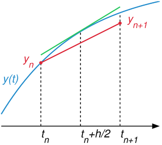
The step size is ${\displaystyle h=1.0}$.

The same illustration for ${\displaystyle h=0.25.}$ The midpoint method converges faster than the Euler method, as ${\displaystyle h\to 0}$.

Numerical methods for ordinary differential equations are methods used to find numerical approximations to the solutions of ordinary differential equations (ODEs). Their use is also known as "numerical integration", although this term can also refer to the computation of integrals.

Many differential equations cannot be solved exactly. For practical purposes, however – such as in engineering – a numeric approximation to the solution is often sufficient. The algorithms studied here can be used to compute such an approximation. An alternative method is to use techniques from calculus to obtain a series expansion of the solution.

Ordinary differential equations occur in many scientific disciplines, including physics, chemistry, biology, and economics. ^[1] In addition, some methods in numerical partial differential equations convert the partial differential equation into an ordinary differential equation, which must then be solved.

The problem

A first-order differential equation is an Initial value problem (IVP) of the form, ^[2]

${\displaystyle y'(t)=f(t,y(t)),\qquad y(t_{0})=y_{0},}$

(1)

where ${\displaystyle f}$ is a function ${\displaystyle f:[t_{0},\infty )\times \mathbb {R} ^{d}\to \mathbb {R} ^{d}}$, and the initial condition ${\displaystyle y_{0}\in \mathbb {R} ^{d}}$ is a given vector. First-order means that only the first derivative of y appears in the equation, and higher derivatives are absent.

Without loss of generality to higher-order systems, we restrict ourselves to first-order differential equations, because a higher-order ODE can be converted into a larger system of first-order equations by introducing extra variables. For example, the second-order equation y′′ = −y can be rewritten as two first-order equations: y′ = z and z′ = −y.

In this section, we describe numerical methods for IVPs, and remark that boundary value problems (BVPs) require a different set of tools. In a BVP, one defines values, or components of the solution y at more than one point. Because of this, different methods need to be used to solve BVPs. For example, the shooting method (and its variants) or global methods like finite differences, ^[3] Galerkin methods, ^[4] or collocation methods are appropriate for that class of problems.

The Picard–Lindelöf theorem states that there is a unique solution, provided f is Lipschitz-continuous.

Methods

Numerical methods for solving first-order IVPs often fall into one of two large categories: ^[5] linear multistep methods, or Runge–Kutta methods. A further division can be realized by dividing methods into those that are explicit and those that are implicit. For example, implicit linear multistep methods include Adams-Moulton methods, and backward differentiation methods (BDF), whereas implicit Runge–Kutta methods ^[6] include diagonally implicit Runge–Kutta (DIRK), ^{[7] [8]} singly diagonally implicit Runge–Kutta (SDIRK), ^[9] and Gauss–Radau ^[10] (based on Gaussian quadrature ^[11] ) numerical methods. Explicit examples from the linear multistep family include the Adams–Bashforth methods, and any Runge–Kutta method with a lower diagonal Butcher tableau is explicit. A loose rule of thumb dictates that stiff differential equations require the use of implicit schemes, whereas non-stiff problems can be solved more efficiently with explicit schemes.

The so-called general linear methods (GLMs) are a generalization of the above two large classes of methods. ^[12]

Euler method

Further information: Euler method

From any point on a curve, you can find an approximation of a nearby point on the curve by moving a short distance along a line tangent to the curve.

Starting with the differential equation ( 1 ), we replace the derivative y′ by the finite difference approximation

${\displaystyle y'(t)\approx {\frac {y(t+h)-y(t)}{h}},}$

(2)

which when re-arranged yields the following formula

${\displaystyle y(t+h)\approx y(t)+hy'(t)}$

and using ( 1 ) gives:

${\displaystyle y(t+h)\approx y(t)+hf(t,y(t)).}$

(3)

This formula is usually applied in the following way. We choose a step size h, and we construct the sequence ${\displaystyle t_{0},t_{1}=t_{0}+h,t_{2}=t_{0}+2h,...}$ We denote by ${\displaystyle y_{n}}$ a numerical estimate of the exact solution ${\displaystyle y(t_{n})}$. Motivated by ( 3 ), we compute these estimates by the following recursive scheme

${\displaystyle y_{n+1}=y_{n}+hf(t_{n},y_{n}).}$

(4)

This is the Euler method (or forward Euler method , in contrast with the backward Euler method, to be described below). The method is named after Leonhard Euler who described it in 1768.

The Euler method is an example of an explicit method. This means that the new value y_n+1 is defined in terms of things that are already known, like y_n.

Backward Euler method

Further information: Backward Euler method

If, instead of ( 2 ), we use the approximation

${\displaystyle y'(t)\approx {\frac {y(t)-y(t-h)}{h}},}$

(5)

we get the backward Euler method:

${\displaystyle y_{n+1}=y_{n}+hf(t_{n+1},y_{n+1}).}$

(6)

The backward Euler method is an implicit method, meaning that we have to solve an equation to find y_n+1. One often uses fixed-point iteration or (some modification of) the Newton–Raphson method to achieve this.

It costs more time to solve this equation than explicit methods; this cost must be taken into consideration when one selects the method to use. The advantage of implicit methods such as ( 6 ) is that they are usually more stable for solving a stiff equation, meaning that a larger step size h can be used.

First-order exponential integrator method

Further information: Exponential integrator

Exponential integrators describe a large class of integrators that have recently seen a lot of development. ^[13] They date back to at least the 1960s.

In place of ( 1 ), we assume the differential equation is either of the form

${\displaystyle y'(t)=-A\,y+{\mathcal {N}}(y),}$

(7)

or it has been locally linearized about a background state to produce a linear term ${\displaystyle -Ay}$ and a nonlinear term ${\displaystyle {\mathcal {N}}(y)}$.

Exponential integrators are constructed by multiplying ( 7 ) by ${\textstyle e^{At}}$, and exactly integrating the result over a time interval ${\displaystyle [t_{n},t_{n+1}=t_{n}+h]}$:

${\displaystyle y_{n+1}=e^{-Ah}y_{n}+\int _{0}^{h}e^{-(h-\tau )A}{\mathcal {N}}\left(y\left(t_{n}+\tau \right)\right)\,d\tau .}$

This integral equation is exact, but it doesn't define the integral.

The first-order exponential integrator can be realized by holding ${\displaystyle {\mathcal {N}}(y(t_{n}+\tau ))}$ constant over the full interval:

${\displaystyle y_{n+1}=e^{-Ah}y_{n}+A^{-1}(1-e^{-Ah}){\mathcal {N}}(y(t_{n}))\ .}$

(8)

Generalizations

The Euler method is often not accurate enough. In more precise terms, it only has order one (the concept of order is explained below). This caused mathematicians to look for higher-order methods.

One possibility is to use not only the previously computed value y_n to determine y_n+1, but to make the solution depend on more past values. This yields a so-called multistep method. Perhaps the simplest is the leapfrog method which is second order and (roughly speaking) relies on two time values.

Almost all practical multistep methods fall within the family of linear multistep methods, which have the form

$${\displaystyle {\begin{aligned}&{}\alpha _{k}y_{n+k}+\alpha _{k-1}y_{n+k-1}+\cdots +\alpha _{0}y_{n}\\&{}\quad =h\left[\beta _{k}f(t_{n+k},y_{n+k})+\beta _{k-1}f(t_{n+k-1},y_{n+k-1})+\cdots +\beta _{0}f(t_{n},y_{n})\right].\end{aligned}}}$$

Another possibility is to use more points in the interval ${\displaystyle [t_{n},t_{n+1}]}$. This leads to the family of Runge–Kutta methods, named after Carl Runge and Martin Kutta. One of their fourth-order methods is especially popular.

Advanced features

A good implementation of one of these methods for solving an ODE entails more than the time-stepping formula.

It is often inefficient to use the same step size all the time, so variable step-size methods have been developed. Usually, the step size is chosen such that the (local) error per step is below some tolerance level. This means that the methods must also compute an error indicator, an estimate of the local error.

An extension of this idea is to choose dynamically between different methods of different orders (this is called a variable order method). Methods based on Richardson extrapolation, ^[14] such as the Bulirsch–Stoer algorithm, ^{[15] [16]} are often used to construct various methods of different orders.

Other desirable features include:

• dense output: cheap numerical approximations for the whole integration interval, and not only at the points t₀, t₁, t₂, ...
• event location: finding the times where, say, a particular function vanishes. This typically requires the use of a root-finding algorithm.
• support for parallel computing.
• when used for integrating with respect to time, time reversibility

Alternative methods

Many methods do not fall within the framework discussed here. Some classes of alternative methods are:

• multiderivative methods, which use not only the function f but also its derivatives. This class includes Hermite–Obreschkoff methods and Fehlberg methods , as well as methods like the Parker–Sochacki method ^[17] or Bychkov–Scherbakov method, which compute the coefficients of the Taylor series of the solution y recursively.
• methods for second order ODEs. We said that all higher-order ODEs can be transformed to first-order ODEs of the form (1). While this is certainly true, it may not be the best way to proceed. In particular, Nyström methods work directly with second-order equations.
• geometric integration methods ^{[18] [19]} are especially designed for special classes of ODEs (for example, symplectic integrators for the solution of Hamiltonian equations). They take care that the numerical solution respects the underlying structure or geometry of these classes.
• Quantized state systems methods are a family of ODE integration methods based on the idea of state quantization. They are efficient when simulating sparse systems with frequent discontinuities.

Parallel-in-time methods

Some IVPs require integration at such high temporal resolution and/or over such long time intervals that classical serial time-stepping methods become computationally infeasible to run in real-time (e.g. IVPs in numerical weather prediction, plasma modelling, and molecular dynamics). Parallel-in-time (PinT) methods have been developed in response to these issues in order to reduce simulation runtimes through the use of parallel computing.

Early PinT methods (the earliest being proposed in the 1960s) ^[20] were initially overlooked by researchers due to the fact that the parallel computing architectures that they required were not yet widely available. With more computing power available, interest was renewed in the early 2000s with the development of Parareal, a flexible, easy-to-use PinT algorithm that is suitable for solving a wide variety of IVPs. The advent of exascale computing has meant that PinT algorithms are attracting increasing research attention and are being developed in such a way that they can harness the world's most powerful supercomputers. The most popular methods as of 2023 include Parareal, PFASST, ParaDiag, and MGRIT. ^[21]

Analysis

Numerical analysis is not only the design of numerical methods, but also their analysis. Three central concepts in this analysis are:

• convergence: whether the method approximates the solution,
• order: how well it approximates the solution, and
• stability: whether errors are damped out. ^[22]

Convergence

Main articles: Sequence, Limit (mathematics), and Limit of a sequence

A numerical method is said to be convergent if the numerical solution approaches the exact solution as the step size h goes to 0. More precisely, we require that for every ODE (1) with a Lipschitz function f and every t^* > 0,

${\displaystyle \lim _{h\to 0^{+}}\max _{n=0,1,\dots ,\lfloor t^{*}/h\rfloor }\left\|y_{n,h}-y(t_{n})\right\|=0.}$

All the methods mentioned above are convergent.

Consistency and order

Further information: Truncation error (numerical integration)

Suppose the numerical method is

${\displaystyle y_{n+k}=\Psi (t_{n+k};y_{n},y_{n+1},\dots ,y_{n+k-1};h).\,}$

The local (truncation) error of the method is the error committed by one step of the method. That is, it is the difference between the result given by the method, assuming that no error was made in earlier steps, and the exact solution:

${\displaystyle \delta _{n+k}^{h}=\Psi \left(t_{n+k};y(t_{n}),y(t_{n+1}),\dots ,y(t_{n+k-1});h\right)-y(t_{n+k}).}$

The method is said to be consistent if

${\displaystyle \lim _{h\to 0}{\frac {\delta _{n+k}^{h}}{h}}=0.}$

The method has order${\displaystyle p}$ if

${\displaystyle \delta _{n+k}^{h}=O(h^{p+1})\quad {\mbox{as }}h\to 0.}$

Hence a method is consistent if it has an order greater than 0. The (forward) Euler method (4) and the backward Euler method (6) introduced above both have order 1, so they are consistent. Most methods being used in practice attain higher order. Consistency is a necessary condition for convergence^{[ citation needed ]}, but not sufficient; for a method to be convergent, it must be both consistent and zero-stable.

A related concept is the global (truncation) error, the error sustained in all the steps one needs to reach a fixed time ${\displaystyle t}$. Explicitly, the global error at time ${\displaystyle t}$ is ${\displaystyle y_{N}-y(t)}$ where ${\displaystyle N=(t-t_{0})/h}$. The global error of a ${\displaystyle p}$th order one-step method is ${\displaystyle O(h^{p})}$; in particular, such a method is convergent. This statement is not necessarily true for multi-step methods.

Stability and stiffness

Further information: Stiff equation

For some differential equations, application of standard methods—such as the Euler method, explicit Runge–Kutta methods, or multistep methods (for example, Adams–Bashforth methods)—exhibit instability in the solutions, though other methods may produce stable solutions. This "difficult behaviour" in the equation (which may not necessarily be complex itself) is described as stiffness, and is often caused by the presence of different time scales in the underlying problem. ^[23] For example, a collision in a mechanical system like in an impact oscillator typically occurs at much smaller time scale than the time for the motion of objects; this discrepancy makes for very "sharp turns" in the curves of the state parameters.

Stiff problems are ubiquitous in chemical kinetics, control theory, solid mechanics, weather forecasting, biology, plasma physics, and electronics. One way to overcome stiffness is to extend the notion of differential equation to that of differential inclusion, which allows for and models non-smoothness. ^{[24] [25]}

History

Below is a timeline of some important developments in this field. ^{[26] [27]}

• 1768 - Leonhard Euler publishes his method.
• 1824 - Augustin Louis Cauchy proves convergence of the Euler method. In this proof, Cauchy uses the implicit Euler method.
• 1855 - First mention of the multistep methods of John Couch Adams in a letter written by Francis Bashforth.
• 1895 - Carl Runge publishes the first Runge–Kutta method.
• 1901 - Martin Kutta describes the popular fourth-order Runge–Kutta method.
• 1910 - Lewis Fry Richardson announces his extrapolation method, Richardson extrapolation.
• 1952 - Charles F. Curtiss and Joseph Oakland Hirschfelder coin the term stiff equations .
• 1963 - Germund Dahlquist introduces A-stability of integration methods.

Numerical solutions to second-order one-dimensional boundary value problems

Boundary value problems (BVPs) are usually solved numerically by solving an approximately equivalent matrix problem obtained by discretizing the original BVP. ^[28] The most commonly used method for numerically solving BVPs in one dimension is called the Finite Difference Method. ^[3] This method takes advantage of linear combinations of point values to construct finite difference coefficients that describe derivatives of the function. For example, the second-order central difference approximation to the first derivative is given by:

${\displaystyle {\frac {u_{i+1}-u_{i-1}}{2h}}=u'(x_{i})+{\mathcal {O}}(h^{2}),}$

and the second-order central difference for the second derivative is given by:

${\displaystyle {\frac {u_{i+1}-2u_{i}+u_{i-1}}{h^{2}}}=u''(x_{i})+{\mathcal {O}}(h^{2}).}$

In both of these formulae, ${\displaystyle h=x_{i}-x_{i-1}}$ is the distance between neighbouring x values on the discretized domain. One then constructs a linear system that can then be solved by standard matrix methods. For example, suppose the equation to be solved is:

${\displaystyle {\begin{aligned}&{}{\frac {d^{2}u}{dx^{2}}}-u=0,\\&{}u(0)=0,\\&{}u(1)=1.\end{aligned}}}$

The next step would be to discretize the problem and use linear derivative approximations such as

${\displaystyle u''_{i}={\frac {u_{i+1}-2u_{i}+u_{i-1}}{h^{2}}}}$

and solve the resulting system of linear equations. This would lead to equations such as:

${\displaystyle {\frac {u_{i+1}-2u_{i}+u_{i-1}}{h^{2}}}-u_{i}=0,\quad \forall i={1,2,3,...,n-1}.}$

On first viewing, this system of equations appears to have difficulty associated with the fact that the equation involves no terms that are not multiplied by variables, but in fact this is false. At i = 1 and n − 1 there is a term involving the boundary values ${\displaystyle u(0)=u_{0}}$ and ${\displaystyle u(1)=u_{n}}$ and since these two values are known, one can simply substitute them into this equation and as a result have a non-homogeneous linear system of equations that has non-trivial solutions.

See also

• Courant–Friedrichs–Lewy condition
• Energy drift
• General linear methods
• List of numerical analysis topics#Numerical methods for ordinary differential equations
• Reversible reference system propagation algorithm
• Modelica Language and OpenModelica software

Notes

1. Chicone, C. (2006). Ordinary differential equations with applications (Vol. 34). Springer Science & Business Media.
2. Bradie (2006 , pp. 533–655)
3. LeVeque, R. J. (2007). Finite difference methods for ordinary and partial differential equations: steady-state and time-dependent problems (Vol. 98). SIAM.
4. Slimane Adjerid and Mahboub Baccouch (2010) Galerkin methods. Scholarpedia, 5(10):10056.
5. Griffiths, D. F., & Higham, D. J. (2010). Numerical methods for ordinary differential equations: initial value problems. Springer Science & Business Media.
6. Hairer, Nørsett & Wanner (1993 , pp. 204–215) harvtxt error: no target: CITEREFHairerNørsettWanner1993 (help)
7. Alexander, R. (1977). Diagonally implicit Runge–Kutta methods for stiff ODE’s. SIAM Journal on Numerical Analysis, 14(6), 1006-1021.
8. Cash, J. R. (1979). Diagonally implicit Runge-Kutta formulae with error estimates. IMA Journal of Applied Mathematics, 24(3), 293-301.
9. Ferracina, L., & Spijker, M. N. (2008). Strong stability of singly-diagonally-implicit Runge–Kutta methods. Applied Numerical Mathematics, 58(11), 1675-1686.
10. Everhart, E. (1985). An efficient integrator that uses Gauss-Radau spacings. In International Astronomical Union Colloquium (Vol. 83, pp. 185-202). Cambridge University Press.
11. Weisstein, Eric W. "Gaussian Quadrature." From MathWorld--A Wolfram Web Resource. https://mathworld.wolfram.com/GaussianQuadrature.html
12. Butcher, J. C. (1987). The numerical analysis of ordinary differential equations: Runge-Kutta and general linear methods. Wiley-Interscience.
13. Hochbruck (2010 , pp. 209–286) harvtxt error: no target: CITEREFHochbruck2010 (help) This is a modern and extensive review paper for exponential integrators
14. Brezinski, C., & Zaglia, M. R. (2013). Extrapolation methods: theory and practice. Elsevier.
15. Monroe, J. L. (2002). Extrapolation and the Bulirsch-Stoer algorithm. Physical Review E, 65(6), 066116.
16. Kirpekar, S. (2003). Implementation of the Bulirsch Stoer extrapolation method. Department of Mechanical Engineering, UC Berkeley/California.
17. Nurminskii, E. A., & Buryi, A. A. (2011). Parker-Sochacki method for solving systems of ordinary differential equations using graphics processors. Numerical Analysis and Applications, 4(3), 223.
18. Hairer, E., Lubich, C., & Wanner, G. (2006). Geometric numerical integration: structure-preserving algorithms for ordinary differential equations (Vol. 31). Springer Science & Business Media.
19. Hairer, E., Lubich, C., & Wanner, G. (2003). Geometric numerical integration illustrated by the Störmer–Verlet method. Acta Numerica, 12, 399-450.
20. Nievergelt, Jürg (1964). "Parallel methods for integrating ordinary differential equations". Communications of the ACM. 7 (12): 731–733. doi: 10.1145/355588.365137 . S2CID   6361754.
21. "Parallel-in-Time.org". Parallel-in-Time.org. Retrieved 15 November 2023.
22. Higham, N. J. (2002). Accuracy and stability of numerical algorithms (Vol. 80). SIAM.
23. Miranker, A. (2001). Numerical Methods for Stiff Equations and Singular Perturbation Problems: and singular perturbation problems (Vol. 5). Springer Science & Business Media.
24. Markus Kunze; Tassilo Kupper (2001). "Non-smooth Dynamical Systems: An Overview". In Bernold Fiedler (ed.). Ergodic Theory, Analysis, and Efficient Simulation of Dynamical Systems. Springer Science & Business Media. p. 431. ISBN   978-3-540-41290-8.
25. Thao Dang (2011). "Model-Based Testing of Hybrid Systems". In Justyna Zander, Ina Schieferdecker and Pieter J. Mosterman (ed.). Model-Based Testing for Embedded Systems. CRC Press. p. 411. ISBN   978-1-4398-1845-9.
26. Brezinski, C., & Wuytack, L. (2012). Numerical analysis: Historical developments in the 20th century. Elsevier.
27. Butcher, J. C. (1996). A history of Runge-Kutta methods. Applied numerical mathematics, 20(3), 247-260.
28. Ascher, U. M., Mattheij, R. M., & Russell, R. D. (1995). Numerical solution of boundary value problems for ordinary differential equations. Society for Industrial and Applied Mathematics.

References

• Bradie, Brian (2006). A Friendly Introduction to Numerical Analysis. Upper Saddle River, New Jersey: Pearson Prentice Hall. ISBN   978-0-13-013054-9.
• J. C. Butcher, Numerical methods for ordinary differential equations, ISBN   0-471-96758-0
• Ernst Hairer, Syvert Paul Nørsett and Gerhard Wanner, Solving ordinary differential equations I: Nonstiff problems, second edition, Springer Verlag, Berlin, 1993. ISBN   3-540-56670-8.
• Ernst Hairer and Gerhard Wanner, Solving ordinary differential equations II: Stiff and differential-algebraic problems, second edition, Springer Verlag, Berlin, 1996. ISBN   3-540-60452-9.
  (This two-volume monograph systematically covers all aspects of the field.)
• Hochbruck, Marlis; Ostermann, Alexander (May 2010). "Exponential integrators". Acta Numerica. 19: 209–286. Bibcode:2010AcNum..19..209H. CiteSeerX   10.1.1.187.6794 . doi:10.1017/S0962492910000048. S2CID   4841957.
• Arieh Iserles, A First Course in the Numerical Analysis of Differential Equations, Cambridge University Press, 1996. ISBN   0-521-55376-8 (hardback), ISBN   0-521-55655-4 (paperback).
  (Textbook, targeting advanced undergraduate and postgraduate students in mathematics, which also discusses numerical partial differential equations.)
• John Denholm Lambert, Numerical Methods for Ordinary Differential Systems, John Wiley & Sons, Chichester, 1991. ISBN   0-471-92990-5.
  (Textbook, slightly more demanding than the book by Iserles.)

External links

• Joseph W. Rudmin, Application of the Parker–Sochacki Method to Celestial Mechanics , 1998.
• Dominique Tournès, L'intégration approchée des équations différentielles ordinaires (1671-1914) , thèse de doctorat de l'université Paris 7 - Denis Diderot, juin 1996. Réimp. Villeneuve d'Ascq : Presses universitaires du Septentrion, 1997, 468 p. (Extensive online material on ODE numerical analysis history, for English-language material on the history of ODE numerical analysis, see, for example, the paper books by Chabert and Goldstine quoted by him.)
• Pchelintsev, A.N. (2020). "An accurate numerical method and algorithm for constructing solutions of chaotic systems". Journal of Applied Nonlinear Dynamics. 9 (2): 207–221. arXiv: 2011.10664 . doi:10.5890/JAND.2020.06.004. S2CID   225853788.
• kv on GitHub (C++ library with rigorous ODE solvers)
• INTLAB (A library made by MATLAB/GNU Octave which includes rigorous ODE solvers)