The derivative is a fundamental tool of calculus that quantifies the sensitivity of change of a function's output with respect to its input. The derivative of a function of a single variable at a chosen input value, when it exists, is the slope of the tangent line to the graph of the function at that point. The tangent line is the best linear approximation of the function near that input value. For this reason, the derivative is often described as the instantaneous rate of change, the ratio of the instantaneous change in the dependent variable to that of the independent variable. The process of finding a derivative is called differentiation.
In mathematics, an equation is a mathematical formula that expresses the equality of two expressions, by connecting them with the equals sign =. The word equation and its cognates in other languages may have subtly different meanings; for example, in French an équation is defined as containing one or more variables, while in English, any well-formed formula consisting of two expressions related with an equals sign is an equation.
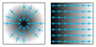
In vector calculus, the gradient of a scalar-valued differentiable function of several variables is the vector field whose value at a point gives the direction and the rate of fastest increase. The gradient transforms like a vector under change of basis of the space of variables of . If the gradient of a function is non-zero at a point , the direction of the gradient is the direction in which the function increases most quickly from , and the magnitude of the gradient is the rate of increase in that direction, the greatest absolute directional derivative. Further, a point where the gradient is the zero vector is known as a stationary point. The gradient thus plays a fundamental role in optimization theory, where it is used to minimize a function by gradient descent. In coordinate-free terms, the gradient of a function may be defined by:

In mathematics, a partial differential equation (PDE) is an equation which computes a function between various partial derivatives of a multivariable function.
In vector calculus, the Jacobian matrix of a vector-valued function of several variables is the matrix of all its first-order partial derivatives. When this matrix is square, that is, when the function takes the same number of variables as input as the number of vector components of its output, its determinant is referred to as the Jacobian determinant. Both the matrix and the determinant are often referred to simply as the Jacobian in literature.
In mathematics, a linear differential equation is a differential equation that is defined by a linear polynomial in the unknown function and its derivatives, that is an equation of the form

In mathematics, separation of variables is any of several methods for solving ordinary and partial differential equations, in which algebra allows one to rewrite an equation so that each of two variables occurs on a different side of the equation.
In mathematics, the method of characteristics is a technique for solving partial differential equations. Typically, it applies to first-order equations, although more generally the method of characteristics is valid for any hyperbolic partial differential equation. The method is to reduce a partial differential equation to a family of ordinary differential equations along which the solution can be integrated from some initial data given on a suitable hypersurface.
In mathematics, the Helmholtz equation is the eigenvalue problem for the Laplace operator. It corresponds to the linear partial differential equation:

In mathematics, a differential equation is an equation that relates one or more unknown functions and their derivatives. In applications, the functions generally represent physical quantities, the derivatives represent their rates of change, and the differential equation defines a relationship between the two. Such relations are common; therefore, differential equations play a prominent role in many disciplines including engineering, physics, economics, and biology.
Numerical methods for partial differential equations is the branch of numerical analysis that studies the numerical solution of partial differential equations (PDEs).
In mathematics, a differential-algebraic system of equations (DAE) is a system of equations that either contains differential equations and algebraic equations, or is equivalent to such a system.
In numerical analysis, the Crank–Nicolson method is a finite difference method used for numerically solving the heat equation and similar partial differential equations. It is a second-order method in time. It is implicit in time, can be written as an implicit Runge–Kutta method, and it is numerically stable. The method was developed by John Crank and Phyllis Nicolson in the mid 20th century.
In mathematics, the convergence condition by Courant–Friedrichs–Lewy is a necessary condition for convergence while solving certain partial differential equations numerically. It arises in the numerical analysis of explicit time integration schemes, when these are used for the numerical solution. As a consequence, the time step must be less than a certain upper bound, given a fixed spatial increment, in many explicit time-marching computer simulations; otherwise, the simulation produces incorrect or unstable results. The condition is named after Richard Courant, Kurt Friedrichs, and Hans Lewy who described it in their 1928 paper.
The method of lines is a technique for solving partial differential equations (PDEs) in which all but one dimension is discretized. By reducing a PDE to a single continuous dimension, the method of lines allows solutions to be computed via methods and software developed for the numerical integration of ordinary differential equations (ODEs) and differential-algebraic systems of equations (DAEs). Many integration routines have been developed over the years in many different programming languages, and some have been published as open source resources.
In numerical analysis, finite-difference methods (FDM) are a class of numerical techniques for solving differential equations by approximating derivatives with finite differences. Both the spatial domain and time domain are discretized, or broken into a finite number of intervals, and the values of the solution at the end points of the intervals are approximated by solving algebraic equations containing finite differences and values from nearby points.

EcosimPro is a simulation tool developed by Empresarios Agrupados A.I.E for modelling simple and complex physical processes that can be expressed in terms of Differential algebraic equations or Ordinary differential equations and Discrete event simulation.
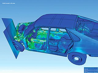
The finite element method (FEM) is a popular method for numerically solving differential equations arising in engineering and mathematical modeling. Typical problem areas of interest include the traditional fields of structural analysis, heat transfer, fluid flow, mass transport, and electromagnetic potential.

In mathematics, an ordinary differential equation (ODE) is a differential equation (DE) dependent on only a single independent variable. As with other DE, its unknown(s) consists of one function(s) and involves the derivatives of those functions. The term "ordinary" is used in contrast with partial differential equations (PDEs) which may be with respect to more than one independent variable, and, less commonly, in contrast with stochastic differential equations (SDEs) where the progression is random.
The Kansa method is a computer method used to solve partial differential equations. Its main advantage is it is very easy to understand and program on a computer. It is much less complicated than the finite element method. Another advantage is it works well on multi variable problems. The finite element method is complicated when working with more than 3 space variables and time.
