
The Navier–Stokes equations are partial differential equations which describe the motion of viscous fluid substances. They were named after French engineer and physicist Claude-Louis Navier and the Irish physicist and mathematician George Gabriel Stokes. They were developed over several decades of progressively building the theories, from 1822 (Navier) to 1842–1850 (Stokes).

In fluid dynamics, the Euler equations are a set of partial differential equations governing adiabatic and inviscid flow. They are named after Leonhard Euler. In particular, they correspond to the Navier–Stokes equations with zero viscosity and zero thermal conductivity.
In fluid mechanics, or more generally continuum mechanics, incompressible flow refers to a flow in which the material density of each fluid parcel — an infinitesimal volume that moves with the flow velocity — is time-invariant. An equivalent statement that implies incompressible flow is that the divergence of the flow velocity is zero.

Smoothed-particle hydrodynamics (SPH) is a computational method used for simulating the mechanics of continuum media, such as solid mechanics and fluid flows. It was developed by Gingold and Monaghan and Lucy in 1977, initially for astrophysical problems. It has been used in many fields of research, including astrophysics, ballistics, volcanology, and oceanography. It is a meshfree Lagrangian method, and the resolution of the method can easily be adjusted with respect to variables such as density.
In numerical methods, total variation diminishing (TVD) is a property of certain discretization schemes used to solve hyperbolic partial differential equations. The most notable application of this method is in computational fluid dynamics. The concept of TVD was introduced by Ami Harten.
In the study of partial differential equations, the MUSCL scheme is a finite volume method that can provide highly accurate numerical solutions for a given system, even in cases where the solutions exhibit shocks, discontinuities, or large gradients. MUSCL stands for Monotonic Upstream-centered Scheme for Conservation Laws, and the term was introduced in a seminal paper by Bram van Leer. In this paper he constructed the first high-order, total variation diminishing (TVD) scheme where he obtained second order spatial accuracy.
Conservation form or Eulerian form refers to an arrangement of an equation or system of equations, usually representing a hyperbolic system, that emphasizes that a property represented is conserved, i.e. a type of continuity equation. The term is usually used in the context of continuum mechanics.
A Riemann problem, named after Bernhard Riemann, is a specific initial value problem composed of a conservation equation together with piecewise constant initial data which has a single discontinuity in the domain of interest. The Riemann problem is very useful for the understanding of equations like Euler conservation equations because all properties, such as shocks and rarefaction waves, appear as characteristics in the solution. It also gives an exact solution to some complex nonlinear equations, such as the Euler equations.
Pressure-correction method is a class of methods used in computational fluid dynamics for numerically solving the Navier-Stokes equations normally for incompressible flows.
In computational fluid dynamics, shock-capturing methods are a class of techniques for computing inviscid flows with shock waves. The computation of flow containing shock waves is an extremely difficult task because such flows result in sharp, discontinuous changes in flow variables such as pressure, temperature, density, and velocity across the shock.
The multiphase particle-in-cell method (MP-PIC) is a numerical method for modeling particle-fluid and particle-particle interactions in a computational fluid dynamics (CFD) calculation. The MP-PIC method achieves greater stability than its particle-in-cell predecessor by simultaneously treating the solid particles as computational particles and as a continuum. In the MP-PIC approach, the particle properties are mapped from the Lagrangian coordinates to an Eulerian grid through the use of interpolation functions. After evaluation of the continuum derivative terms, the particle properties are mapped back to the individual particles. This method has proven to be stable in dense particle flows, computationally efficient, and physically accurate. This has allowed the MP-PIC method to be used as particle-flow solver for the simulation of industrial-scale chemical processes involving particle-fluid flows.
In computational fluid dynamics QUICK, which stands for Quadratic Upstream Interpolation for Convective Kinematics, is a higher-order differencing scheme that considers a three-point upstream weighted by quadratic interpolation for the cell face values. In computational fluid dynamics there are many solution methods for solving the steady convection–diffusion equation. Some of the used methods are the central differencing scheme, upwind scheme, hybrid scheme, power law scheme and QUICK scheme.
The hybrid difference scheme is a method used in the numerical solution for convection–diffusion problems. It was introduced by Spalding (1970). It is a combination of central difference scheme and upwind difference scheme as it exploits the favorable properties of both of these schemes.
False diffusion is a type of error observed when the upwind scheme is used to approximate the convection term in convection–diffusion equations. The more accurate central difference scheme can be used for the convection term, but for grids with cell Peclet number more than 2, the central difference scheme is unstable and the simpler upwind scheme is often used. The resulting error from the upwind differencing scheme has a diffusion-like appearance in two- or three-dimensional co-ordinate systems and is referred as "false diffusion". False-diffusion errors in numerical solutions of convection-diffusion problems, in two- and three-dimensions, arise from the numerical approximations of the convection term in the conservation equations. Over the past 20 years many numerical techniques have been developed to solve convection-diffusion equations and none are problem-free, but false diffusion is one of the most serious problems and a major topic of controversy and confusion among numerical analysts.
The Finite volume method in computational fluid dynamics is a discretization technique for partial differential equations that arise from physical conservation laws. These equations can be different in nature, e.g. elliptic, parabolic, or hyperbolic. The first well-documented use of this method was by Evans and Harlow (1957) at Los Alamos. The general equation for steady diffusion can easily be derived from the general transport equation for property Φ by deleting transient and convective terms.
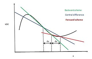
In applied mathematics, the central differencing scheme is a finite difference method that optimizes the approximation for the differential operator in the central node of the considered patch and provides numerical solutions to differential equations. It is one of the schemes used to solve the integrated convection–diffusion equation and to calculate the transported property Φ at the e and w faces, where e and w are short for east and west. The method's advantages are that it is easy to understand and implement, at least for simple material relations; and that its convergence rate is faster than some other finite differencing methods, such as forward and backward differencing. The right side of the convection-diffusion equation, which basically highlights the diffusion terms, can be represented using central difference approximation. To simplify the solution and analysis, linear interpolation can be used logically to compute the cell face values for the left side of this equation, which is nothing but the convective terms. Therefore, cell face values of property for a uniform grid can be written as:
Unsteady flows are characterized as flows in which the properties of the fluid are time dependent. It gets reflected in the governing equations as the time derivative of the properties are absent. For Studying Finite-volume method for unsteady flow there is some governing equations >
The upwind differencing scheme is a method used in numerical methods in computational fluid dynamics for convection–diffusion problems. This scheme is specific for Peclet number greater than 2 or less than −2
The convection–diffusion equation describes the flow of heat, particles, or other physical quantities in situations where there is both diffusion and convection or advection. For information about the equation, its derivation, and its conceptual importance and consequences, see the main article convection–diffusion equation. This article describes how to use a computer to calculate an approximate numerical solution of the discretized equation, in a time-dependent situation.
Finite volume method (FVM) is a numerical method. FVM in computational fluid dynamics is used to solve the partial differential equation which arises from the physical conservation law by using discretisation. Convection is always followed by diffusion and hence where convection is considered we have to consider combine effect of convection and diffusion. But in places where fluid flow plays a non-considerable role we can neglect the convective effect of the flow. In this case we have to consider more simplistic case of only diffusion. The general equation for steady convection-diffusion can be easily derived from the general transport equation for property by deleting transient.


