Exponential response formula

Last updated

In mathematics, the exponential response formula (ERF), also known as exponential response and complex replacement, is a method used to find a particular solution of a non-homogeneous linear ordinary differential equation of any order. [1] [2] The exponential response formula is applicable to non-homogeneous linear ordinary differential equations with constant coefficients if the function is polynomial, sinusoidal, exponential or the combination of the three. [2] The general solution of a non-homogeneous linear ordinary differential equation is a superposition of the general solution of the associated homogeneous ODE and a particular solution to the non-homogeneous ODE. [1] Alternative methods for solving ordinary differential equations of higher order are method of undetermined coefficients and method of variation of parameters.

Contents

Context and method

Applicability

The ERF method of finding a particular solution of a non-homogeneous differential equation is applicable if the non-homogeneous equation is or could be transformed to form ; where are real or complex numbers and is homogeneous linear differential equation of any order. Then, the exponential response formula can be applied to each term of the right side of such equation. Due to linearity, the exponential response formula can be applied as long as the right side has terms, which are added together by the superposition principle.

Complex replacement

Complex replacement is a method of converting a non-homogeneous term of equation into a complex exponential function, which makes a given differential equation a complex exponential.

Consider differential equation .

To make complex replacement, Euler's formula can be used;

Therefore, given differential equation changes to . The solution of the complex differential equation can be found as , from which the real part is the solution of the original equation.

Complex replacement is used for solving differential equations when the non-homogeneous term is expressed in terms of a sinusoidal function or an exponential function, which can be converted into a complex exponential function differentiation and integration. Such complex exponential function is easier to manipulate than the original function.

When the non-homogeneous term is expressed as an exponential function, the ERF method or the undetermined coefficients method can be used to find a particular solution. If non-homogeneous terms can not be transformed to complex exponential function, then the Lagrange method of variation of parameters can be used to find solutions.

Linear time-invariant operator

The differential equations are important in simulating natural phenomena. In particular, there are numerous phenomena described as high order linear differential equations, for example the spring vibration, LRC circuit, beam deflection, signal processing, control theory and LTI systems with feedback loops. [1] [3]

Mathematically, the system is time-invariant if whenever the input has response then for any constant "a", the input has response . Physically, time invariance means system’s response does not depend on what time the input begins. For example, if a spring-mass system is at equilibrium, it will respond to a given force in the same way, no matter when the force was applied.

When the time-invariant system is also linear, it is called a linear time-invariant system (LTI system). Most of these LTI systems are derived from linear differential equations, where the non-homogeneous term is called the input signal and solution of the non-homogeneous equations is called the response signal. If the input signal is given exponentially, the corresponding response signal also changes exponentially.

Considering the following th order linear differential equation

and denoting

where are the constant coefficients, produces differential operator , which is linear and time-invariant and known as the LTI operator. The operator, is obtained from its characteristic polynomial;

by formally replacing the indeterminate s here with the differentiation operator

Therefore, the equation (1) can be written as

Problem setting and ERF method

Considering LTI differential equation above, with exponential input , where and are given numbers. Then, a particular solution is

provide only that .

Proof: Due to linearity of operator , the equation can be written as

On the other hand, since

substituting this into equation (3), produces

Therefore, is a particular solution to the non-homogeneous differential equation.

Thus, the above equation for a particular response is called the exponential response formula (ERF) for the given exponential input.

In particular, in case of , a solution to equation (2) is given by

and is called the resonant response formula.

Example

Let's find the particular solution to 2nd order linear non-homogeneous ODE;

The characteristic polynomial is . Also, the non-homogeneous term, can be written as follows

Then, the particular solutions corresponding to and , are found, respectively.

First, considering non-homogeneous term, . In this case, since and .

from the ERF, a particular solution corresponding to can be found.

.

Similarly, a particular solution can be found corresponding to .

Let's find a particular solution to DE corresponding to 3rd term;

In order to do this, equation must be replaced by complex-valued equation, of which it is the real part:

Applying the exponential response formula (ERF), produces

and the real part is

Therefore, the particular solution of given equation, is

Comparison with method of undetermined coefficients

The undetermined coefficients method is a method of appropriately selecting a solution type according to the form of the non-homogeneous term and determining the undetermined constant, so that it satisfies the non-homogeneous equation. [4] On the other hand, the ERF method obtains a special solution based on differential operator. [2] Similarity for both methods is that special solutions of non-homogeneous linear differential equations with constant coefficients are obtained, while form of the equation in consideration is the same in both methods.

For example, finding a particular solution of with the method of undetermined coefficients requires solving the characteristic equation . The non-homogeneous term is then considered and since is not a characteristic root, it puts a particular solution in form of , where is undetermined constant. Substituting into the equation to determine the tentative constant yields

therefore

The particular solution can be found in form: [5]

On the other hand, the exponential response formula method requires characteristic polynomial to be found, after which the non-homogeneous terms is complex replaced. The particular solution is then found using formula

Generalized exponential response formula

The exponential response formula method was discussed in case of . In the case of , the resonant response formula is also considered.

In the case of , we will discuss how the ERF method will be described in this section.

Let be a polynomial operator with constant coefficients, and its -th derivative. Then ODE

, where is real or complex.

has the particular solution as following.

Above equation is called generalized exponential response formula.

Example

To find a particular solution of the following ODE;

the characteristic polynomial is .

By the calculating, we get the following:

Original exponential response formula is not applicable to this case due to division by zero. Therefore, using the generalized exponential response formula and calculated constants, particular solution is

Application examples

Motion of object hanging from a spring

Object hanging from a spring with displacement . The force acting is gravity, spring force, air resistance, and any other external forces.

From Hooke’s law, the motion equation of object is expressed as follows; [6] [4]

where is external force.

Now, assuming drag is neglected and , where (the external force frequency coincides with the natural frequency). Therefore, the harmonic oscillator with sinusoidal forcing term is expressed as following:

Then, a particular solution is

Applying complex replacement and the ERF: if is a solution to the complex DE

then will be a solution to the given DE.

The characteristic polynomial is , and , so that . However, since , then . Thus, the resonant case of the ERF gives

Electrical circuits

Considering the electric current flowing through an electric circuit, consisting of a resistance (), a capacitor (), a coil wires (), and a battery (), connected in series. [3] [6]

This system is described by an integral-differential equation found by Kirchhoff called Kirchhoff’s voltage law, relating the resistor , capacitor , inductor , battery , and the current in a circuit as follows,

Differentiating both sides of the above equation, produces the following ODE.

Now, assuming , where . ( is called resonance frequency in LRC circuit). Under above assumption, the output (particular solution) corresponding to input can be found. In order to do it, given input can be converted in complex form:

The characteristic polynomial is , where . Therefore, from the ERF, a particular solution can be obtained as follows;

Complex gain and phase lag

Considering the general LTI system

where is the input and are given polynomial operators, while assuming that . In case that , a particular solution to given equation is

Considering the following concepts used in physics and signal processing mainly.

Related Research Articles

In classical mechanics, a harmonic oscillator is a system that, when displaced from its equilibrium position, experiences a restoring force F proportional to the displacement x:

<span class="mw-page-title-main">Oscillation</span> Repetitive variation of some measure about a central value

Oscillation is the repetitive or periodic variation, typically in time, of some measure about a central value or between two or more different states. Familiar examples of oscillation include a swinging pendulum and alternating current. Oscillations can be used in physics to approximate complex interactions, such as those between atoms.

<span class="mw-page-title-main">Polar coordinate system</span> Coordinates determined by distance and angle

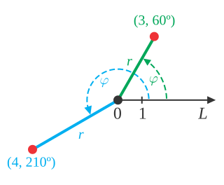
In mathematics, the polar coordinate system is a two-dimensional coordinate system in which each point on a plane is determined by a distance from a reference point and an angle from a reference direction. The reference point is called the pole, and the ray from the pole in the reference direction is the polar axis. The distance from the pole is called the radial coordinate, radial distance or simply radius, and the angle is called the angular coordinate, polar angle, or azimuth. Angles in polar notation are generally expressed in either degrees or radians.

<span class="mw-page-title-main">Navier–Stokes equations</span> Equations describing the motion of viscous fluid substances

The Navier–Stokes equations are partial differential equations which describe the motion of viscous fluid substances. They were named after French engineer and physicist Claude-Louis Navier and the Irish physicist and mathematician George Gabriel Stokes. They were developed over several decades of progressively building the theories, from 1822 (Navier) to 1842–1850 (Stokes).

In calculus, and more generally in mathematical analysis, integration by parts or partial integration is a process that finds the integral of a product of functions in terms of the integral of the product of their derivative and antiderivative. It is frequently used to transform the antiderivative of a product of functions into an antiderivative for which a solution can be more easily found. The rule can be thought of as an integral version of the product rule of differentiation.

<span class="mw-page-title-main">Spherical harmonics</span> Special mathematical functions defined on the surface of a sphere

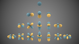
In mathematics and physical science, spherical harmonics are special functions defined on the surface of a sphere. They are often employed in solving partial differential equations in many scientific fields.

The sine-Gordon equation is a nonlinear hyperbolic partial differential equation for a function dependent on two variables typically denoted and , involving the wave operator and the sine of .

In physics, Liouville's theorem, named after the French mathematician Joseph Liouville, is a key theorem in classical statistical and Hamiltonian mechanics. It asserts that the phase-space distribution function is constant along the trajectories of the system—that is that the density of system points in the vicinity of a given system point traveling through phase-space is constant with time. This time-independent density is in statistical mechanics known as the classical a priori probability.

In physics, the Hamilton–Jacobi equation, named after William Rowan Hamilton and Carl Gustav Jacob Jacobi, is an alternative formulation of classical mechanics, equivalent to other formulations such as Newton's laws of motion, Lagrangian mechanics and Hamiltonian mechanics.

In rotordynamics, the rigid rotor is a mechanical model of rotating systems. An arbitrary rigid rotor is a 3-dimensional rigid object, such as a top. To orient such an object in space requires three angles, known as Euler angles. A special rigid rotor is the linear rotor requiring only two angles to describe, for example of a diatomic molecule. More general molecules are 3-dimensional, such as water, ammonia, or methane.

In mathematics and physics, the Christoffel symbols are an array of numbers describing a metric connection. The metric connection is a specialization of the affine connection to surfaces or other manifolds endowed with a metric, allowing distances to be measured on that surface. In differential geometry, an affine connection can be defined without reference to a metric, and many additional concepts follow: parallel transport, covariant derivatives, geodesics, etc. also do not require the concept of a metric. However, when a metric is available, these concepts can be directly tied to the "shape" of the manifold itself; that shape is determined by how the tangent space is attached to the cotangent space by the metric tensor. Abstractly, one would say that the manifold has an associated (orthonormal) frame bundle, with each "frame" being a possible choice of a coordinate frame. An invariant metric implies that the structure group of the frame bundle is the orthogonal group O(p, q). As a result, such a manifold is necessarily a (pseudo-)Riemannian manifold. The Christoffel symbols provide a concrete representation of the connection of (pseudo-)Riemannian geometry in terms of coordinates on the manifold. Additional concepts, such as parallel transport, geodesics, etc. can then be expressed in terms of Christoffel symbols.

<span class="mw-page-title-main">Duffing equation</span> Non-linear second order differential equation and its attractor

The Duffing equation, named after Georg Duffing (1861–1944), is a non-linear second-order differential equation used to model certain damped and driven oscillators. The equation is given by

A theoretical motivation for general relativity, including the motivation for the geodesic equation and the Einstein field equation, can be obtained from special relativity by examining the dynamics of particles in circular orbits about the Earth. A key advantage in examining circular orbits is that it is possible to know the solution of the Einstein Field Equation a priori. This provides a means to inform and verify the formalism.

The gradient theorem, also known as the fundamental theorem of calculus for line integrals, says that a line integral through a gradient field can be evaluated by evaluating the original scalar field at the endpoints of the curve. The theorem is a generalization of the second fundamental theorem of calculus to any curve in a plane or space rather than just the real line.

In the differential geometry of surfaces, a Darboux frame is a natural moving frame constructed on a surface. It is the analog of the Frenet–Serret frame as applied to surface geometry. A Darboux frame exists at any non-umbilic point of a surface embedded in Euclidean space. It is named after French mathematician Jean Gaston Darboux.

In physics and chemistry, specifically in nuclear magnetic resonance (NMR), magnetic resonance imaging (MRI), and electron spin resonance (ESR), the Bloch equations are a set of macroscopic equations that are used to calculate the nuclear magnetization M = (Mx, My, Mz) as a function of time when relaxation times T1 and T2 are present. These are phenomenological equations that were introduced by Felix Bloch in 1946. Sometimes they are called the equations of motion of nuclear magnetization. They are analogous to the Maxwell–Bloch equations.

An electric dipole transition is the dominant effect of an interaction of an electron in an atom with the electromagnetic field.

The narrow escape problem is a ubiquitous problem in biology, biophysics and cellular biology.

In mathematics, a linear recurrence with constant coefficients sets equal to 0 a polynomial that is linear in the various iterates of a variable—that is, in the values of the elements of a sequence. The polynomial's linearity means that each of its terms has degree 0 or 1. A linear recurrence denotes the evolution of some variable over time, with the current time period or discrete moment in time denoted as t, one period earlier denoted as t − 1, one period later as t + 1, etc.

<span class="mw-page-title-main">Stokes problem</span>

In fluid dynamics, Stokes problem also known as Stokes second problem or sometimes referred to as Stokes boundary layer or Oscillating boundary layer is a problem of determining the flow created by an oscillating solid surface, named after Sir George Stokes. This is considered one of the simplest unsteady problems that has an exact solution for the Navier-Stokes equations. In turbulent flow, this is still named a Stokes boundary layer, but now one has to rely on experiments, numerical simulations or approximate methods in order to obtain useful information on the flow.

References

  1. 1 2 3 Miller, Haynes; Mattuck, Arthur (June 2004), Differential Equations, vol. IMSCP-MD5-9ca77abee86dc4bbaef9e2d6b157eaa9, pp. 50–56, hdl:1721.1/34888
  2. 1 2 3 Wirkus, Stephen A.; Swift, Randal J.; Szypowski, Ryan S. (2016), A Course in Differential Equations with Boundary Value Problems, Second Edition, Textbooks in Mathematics (2nd ed.), Chapman and Hall/CRC, pp. 230–238, ISBN   978-1498736053
  3. 1 2 Charles L, Phillips (2007), Signals, Systems, And Transforms, Prentice Hall, pp. 112–122, ISBN   978-0-13-198923-8
  4. 1 2 Coddington, Earl A.; Carlson, Robert (1997), Linear Ordinary Differential Equations (PDF), pp. 3–80, ISBN   0-89871-388-9
  5. Ralph P. Grimaldi (2000). "Nonhomogeneous Recurrence Relations". Section 3.3.3 of Handbook of Discrete and Combinatorial Mathematics. Kenneth H. Rosen, ed. CRC Press. ISBN   0-8493-0149-1.
  6. 1 2 Edwards, C. Henry; Penney, David E. (2008), ELEMENTARY DIFFERENTIAL EQUATIONS, Pearson Prentice Hall, pp. 100–193, ISBN   978-0-13-239730-8