Jet bundle

"Jet space" redirects here. Not to be confused with space jet.

In differential topology, the jet bundle is a certain construction that makes a new smooth fiber bundle out of a given smooth fiber bundle. It makes it possible to write differential equations on sections of a fiber bundle in an invariant form. Jets may also be seen as the coordinate free versions of Taylor expansions.

Historically, jet bundles are attributed to Charles Ehresmann, and were an advance on the method (prolongation) of Élie Cartan, of dealing geometrically with higher derivatives, by imposing differential form conditions on newly introduced formal variables. Jet bundles are sometimes called sprays, although sprays usually refer more specifically to the associated vector field induced on the corresponding bundle (e.g., the geodesic spray on Finsler manifolds.)

Since the early 1980s, jet bundles have appeared as a concise way to describe phenomena associated with the derivatives of maps, particularly those associated with the calculus of variations. ^[1] Consequently, the jet bundle is now recognized as the correct domain for a geometrical covariant field theory and much work is done in general relativistic formulations of fields using this approach.

Jets

Main article: Jet (mathematics)

Suppose M is an m-dimensional manifold and that (E, π, M) is a fiber bundle. For p ∈ M, let Γ(p) denote the set of all local sections whose domain contains p. Let ${\displaystyle I=(I(1),I(2),...,I(m))}$ be a multi-index (an m-tuple of non-negative integers, not necessarily in ascending order), then define:

${\displaystyle {\begin{aligned}|I|&:=\sum _{i=1}^{m}I(i)\\{\frac {\partial ^{|I|}}{\partial x^{I}}}&:=\prod _{i=1}^{m}\left({\frac {\partial }{\partial x^{i}}}\right)^{I(i)}.\end{aligned}}}$

Define the local sections σ, η ∈ Γ(p) to have the same r-jet at p if

${\displaystyle \left.{\frac {\partial ^{|I|}\sigma ^{\alpha }}{\partial x^{I}}}\right|_{p}=\left.{\frac {\partial ^{|I|}\eta ^{\alpha }}{\partial x^{I}}}\right|_{p},\quad 0\leq |I|\leq r.}$

The relation that two maps have the same r-jet is an equivalence relation. An r-jet is an equivalence class under this relation, and the r-jet with representative σ is denoted ${\displaystyle j_{p}^{r}\sigma }$. The integer r is also called the order of the jet, p is its source and σ(p) is its target.

Jet manifolds

The r-th jet manifold of π is the set

${\displaystyle J^{r}(\pi )=\left\{j_{p}^{r}\sigma :p\in M,\sigma \in \Gamma (p)\right\}.}$

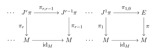
We may define projections π_r and π_r,0 called the source and target projections respectively, by

${\displaystyle {\begin{cases}\pi _{r}:J^{r}(\pi )\to M\\j_{p}^{r}\sigma \mapsto p\end{cases}},\qquad {\begin{cases}\pi _{r,0}:J^{r}(\pi )\to E\\j_{p}^{r}\sigma \mapsto \sigma (p)\end{cases}}}$

If 1 ≤ k ≤ r, then the k-jet projection is the function π_r,k defined by

${\displaystyle {\begin{cases}\pi _{r,k}:J^{r}(\pi )\to J^{k}(\pi )\\j_{p}^{r}\sigma \mapsto j_{p}^{k}\sigma \end{cases}}}$

From this definition, it is clear that π_r = π o π_r,0 and that if 0 ≤ m ≤ k, then π_r,m = π_k,m o π_r,k. It is conventional to regard π_r,r as the identity map on J ^r(π) and to identify J ⁰(π) with E.

The functions π_r,k, π_r,0 and π_r are smooth surjective submersions.

A coordinate system on E will generate a coordinate system on J ^r(π). Let (U, u) be an adapted coordinate chart on E, where u = (xⁱ, u^α). The induced coordinate chart (U^r, u^r) on J ^r(π) is defined by

${\displaystyle {\begin{aligned}U^{r}&=\left\{j_{p}^{r}\sigma :p\in M,\sigma (p)\in U\right\}\\u^{r}&=\left(x^{i},u^{\alpha },u_{I}^{\alpha }\right)\end{aligned}}}$

where

${\displaystyle {\begin{aligned}x^{i}\left(j_{p}^{r}\sigma \right)&=x^{i}(p)\\u^{\alpha }\left(j_{p}^{r}\sigma \right)&=u^{\alpha }(\sigma (p))\end{aligned}}}$

and the ${\displaystyle n\left({\binom {m+r}{r}}-1\right)}$ functions known as the derivative coordinates:

${\displaystyle {\begin{cases}u_{I}^{\alpha }:U^{k}\to \mathbf {R} \\u_{I}^{\alpha }\left(j_{p}^{r}\sigma \right)=\left.{\frac {\partial ^{|I|}\sigma ^{\alpha }}{\partial x^{I}}}\right|_{p}\end{cases}}}$

Given an atlas of adapted charts (U, u) on E, the corresponding collection of charts (U ^r, u ^r) is a finite-dimensional C^∞ atlas on J ^r(π).

Jet bundles

Since the atlas on each ${\displaystyle J^{r}(\pi )}$ defines a manifold, the triples ${\displaystyle (J^{r}(\pi ),\pi _{r,k},J^{k}(\pi ))}$, ${\displaystyle (J^{r}(\pi ),\pi _{r,0},E)}$ and ${\displaystyle (J^{r}(\pi ),\pi _{r},M)}$ all define fibered manifolds. In particular, if ${\displaystyle (E,\pi ,M)}$is a fiber bundle, the triple ${\displaystyle (J^{r}(\pi ),\pi _{r},M)}$ defines the r-th jet bundle of π.

If W ⊂ M is an open submanifold, then

${\displaystyle J^{r}\left(\pi |_{\pi ^{-1}(W)}\right)\cong \pi _{r}^{-1}(W).\,}$

If p ∈ M, then the fiber ${\displaystyle \pi _{r}^{-1}(p)\,}$ is denoted ${\displaystyle J_{p}^{r}(\pi )}$.

Let σ be a local section of π with domain W ⊂ M. The r-th jet prolongation of σ is the map ${\displaystyle j^{r}\sigma :W\rightarrow J^{r}(\pi )}$ defined by

${\displaystyle (j^{r}\sigma )(p)=j_{p}^{r}\sigma .\,}$

Note that ${\displaystyle \pi _{r}\circ j^{r}\sigma =\mathbb {id} _{W}}$, so ${\displaystyle j^{r}\sigma }$ really is a section. In local coordinates, ${\displaystyle j^{r}\sigma }$ is given by

${\displaystyle \left(\sigma ^{\alpha },{\frac {\partial ^{|I|}\sigma ^{\alpha }}{\partial x^{I}}}\right)\qquad 1\leq |I|\leq r.\,}$

We identify ${\displaystyle j^{0}\sigma }$ with ${\displaystyle \sigma }$ .

Algebro-geometric perspective

An independently motivated construction of the sheaf of sections ${\displaystyle \Gamma J^{k}\left(\pi _{TM}\right)}$ is given.

Consider a diagonal map ${\textstyle \Delta _{n}:M\to \prod _{i=1}^{n+1}M}$, where the smooth manifold ${\displaystyle M}$ is a locally ringed space by ${\displaystyle C^{k}(U)}$ for each open ${\displaystyle U}$. Let ${\displaystyle {\mathcal {I}}}$ be the ideal sheaf of ${\displaystyle \Delta _{n}(M)}$, equivalently let ${\displaystyle {\mathcal {I}}}$ be the sheaf of smooth germs which vanish on ${\displaystyle \Delta _{n}(M)}$ for all ${\displaystyle 0<n\leq k}$. The pullback of the quotient sheaf ${\displaystyle {\Delta _{n}}^{*}\left({\mathcal {I}}/{\mathcal {I}}^{n+1}\right)}$ from ${\textstyle \prod _{i=1}^{n+1}M}$ to ${\displaystyle M}$ by ${\displaystyle \Delta _{n}}$ is the sheaf of k-jets. ^[2]

The direct limit of the sequence of injections given by the canonical inclusions ${\displaystyle {\mathcal {I}}^{n+1}\hookrightarrow {\mathcal {I}}^{n}}$ of sheaves, gives rise to the infinite jet sheaf${\displaystyle {\mathcal {J}}^{\infty }(TM)}$. Observe that by the direct limit construction it is a filtered ring.

Example

If π is the trivial bundle (M × R, pr₁, M), then there is a canonical diffeomorphism between the first jet bundle ${\displaystyle J^{1}(\pi )}$ and T*M × R. To construct this diffeomorphism, for each σ in ${\displaystyle \Gamma _{M}(\pi )}$ write ${\displaystyle {\bar {\sigma }}=pr_{2}\circ \sigma \in C^{\infty }(M)\,}$.

Then, whenever p ∈ M

${\displaystyle j_{p}^{1}\sigma =\left\{\psi$ :\psi \in \Gamma _{p}(\pi );{\bar {\psi }}(p)={\bar {\sigma }}(p);d{\bar {\psi }}_{p}=d{\bar {\sigma }}_{p}\right\}.\,}

Consequently, the mapping

${\displaystyle {\begin{cases}J^{1}(\pi )\to T^{*}M\times \mathbf {R} \\j_{p}^{1}\sigma \mapsto \left(d{\bar {\sigma }}_{p},{\bar {\sigma }}(p)\right)\end{cases}}}$

is well-defined and is clearly injective. Writing it out in coordinates shows that it is a diffeomorphism, because if (xⁱ, u) are coordinates on M × R, where u = id_R is the identity coordinate, then the derivative coordinates u_i on J¹(π) correspond to the coordinates ∂_i on T*M.

Likewise, if π is the trivial bundle (R × M, pr₁, R), then there exists a canonical diffeomorphism between ${\displaystyle J^{1}(\pi )}$and R × TM.

Contact structure

The space J^r(π) carries a natural distribution, that is, a sub-bundle of the tangent bundle TJ^r(π)), called the Cartan distribution. The Cartan distribution is spanned by all tangent planes to graphs of holonomic sections; that is, sections of the form j^rφ for φ a section of π.

The annihilator of the Cartan distribution is a space of differential one-forms called contact forms, on J^r(π). The space of differential one-forms on J^r(π) is denoted by ${\displaystyle \Lambda ^{1}J^{r}(\pi )}$ and the space of contact forms is denoted by ${\displaystyle \Lambda _{C}^{r}\pi }$. A one form is a contact form provided its pullback along every prolongation is zero. In other words, ${\displaystyle \theta \in \Lambda ^{1}J^{r}\pi }$ is a contact form if and only if

${\displaystyle \left(j^{r+1}\sigma \right)^{*}\theta =0}$

for all local sections σ of π over M.

The Cartan distribution is the main geometrical structure on jet spaces and plays an important role in the geometric theory of partial differential equations. The Cartan distributions are completely non-integrable. In particular, they are not involutive. The dimension of the Cartan distribution grows with the order of the jet space. However, on the space of infinite jets J^∞ the Cartan distribution becomes involutive and finite-dimensional: its dimension coincides with the dimension of the base manifold M.

Example

Consider the case (E, π, M), where E ≃ R² and M ≃ R. Then, (J¹(π), π, M) defines the first jet bundle, and may be coordinated by (x, u, u₁), where

${\displaystyle {\begin{aligned}x\left(j_{p}^{1}\sigma \right)&=x(p)=x\\u\left(j_{p}^{1}\sigma \right)&=u(\sigma (p))=u(\sigma (x))=\sigma (x)\\u_{1}\left(j_{p}^{1}\sigma \right)&=\left.{\frac {\partial \sigma }{\partial x}}\right|_{p}=\sigma '(x)\end{aligned}}}$

for all p ∈ M and σ in Γ_p(π). A general 1-form on J¹(π) takes the form

${\displaystyle \theta =a(x,u,u_{1})dx+b(x,u,u_{1})du+c(x,u,u_{1})du_{1}\,}$

A section σ in Γ_p(π) has first prolongation

${\displaystyle j^{1}\sigma =(u,u_{1})=\left(\sigma (p),\left.{\frac {\partial \sigma }{\partial x}}\right|_{p}\right).}$

Hence, (j¹σ)*θ can be calculated as

${\displaystyle {\begin{aligned}\left(j_{p}^{1}\sigma \right)^{*}\theta &=\theta \circ j_{p}^{1}\sigma \\&=a(x,\sigma (x),\sigma '(x))dx+b(x,\sigma (x),\sigma '(x))d(\sigma (x))+c(x,\sigma (x),\sigma '(x))d(\sigma '(x))\\&=a(x,\sigma (x),\sigma '(x))dx+b(x,\sigma (x),\sigma '(x))\sigma '(x)dx+c(x,\sigma (x),\sigma '(x))\sigma ''(x)dx\\&=[a(x,\sigma (x),\sigma '(x))+b(x,\sigma (x),\sigma '(x))\sigma '(x)+c(x,\sigma (x),\sigma '(x))\sigma ''(x)]dx\end{aligned}}}$

This will vanish for all sections σ if and only if c = 0 and a = −bσ′(x). Hence, θ = b(x, u, u₁)θ₀ must necessarily be a multiple of the basic contact form θ₀ = du − u₁dx. Proceeding to the second jet space J²(π) with additional coordinate u₂, such that

${\displaystyle u_{2}(j_{p}^{2}\sigma )=\left.{\frac {\partial ^{2}\sigma }{\partial x^{2}}}\right|_{p}=\sigma ''(x)\,}$

a general 1-form has the construction

${\displaystyle \theta =a(x,u,u_{1},u_{2})dx+b(x,u,u_{1},u_{2})du+c(x,u,u_{1},u_{2})du_{1}+e(x,u,u_{1},u_{2})du_{2}\,}$

This is a contact form if and only if

${\displaystyle {\begin{aligned}\left(j_{p}^{2}\sigma \right)^{*}\theta &=\theta \circ j_{p}^{2}\sigma \\&=a(x,\sigma (x),\sigma '(x),\sigma ''(x))dx+b(x,\sigma (x),\sigma '(x),\sigma ''(x))d(\sigma (x))+{}\\&\qquad \qquad c(x,\sigma (x),\sigma '(x),\sigma ''(x))d(\sigma '(x))+e(x,\sigma (x),\sigma '(x),\sigma ''(x))d(\sigma ''(x))\\&=adx+b\sigma '(x)dx+c\sigma ''(x)dx+e\sigma '''(x)dx\\&=[a+b\sigma '(x)+c\sigma ''(x)+e\sigma '''(x)]dx\\&=0\end{aligned}}}$

which implies that e = 0 and a = −bσ′(x) − cσ′′(x). Therefore, θ is a contact form if and only if

${\displaystyle \theta =b(x,\sigma (x),\sigma '(x))\theta _{0}+c(x,\sigma (x),\sigma '(x))\theta _{1},}$

where θ₁ = du₁ − u₂dx is the next basic contact form (Note that here we are identifying the form θ₀ with its pull-back ${\displaystyle \left(\pi _{2,1}\right)^{*}\theta _{0}}$ to J²(π)).

In general, providing x, u ∈ R, a contact form on J^r+1(π) can be written as a linear combination of the basic contact forms

${\displaystyle \theta _{k}=du_{k}-u_{k+1}dx\qquad k=0,\ldots ,r-1\,}$

where

${\displaystyle u_{k}\left(j^{k}\sigma \right)=\left.{\frac {\partial ^{k}\sigma }{\partial x^{k}}}\right|_{p}.}$

Similar arguments lead to a complete characterization of all contact forms.

In local coordinates, every contact one-form on J^r+1(π) can be written as a linear combination

${\displaystyle \theta =\sum _{|I|=0}^{r}P_{\alpha }^{I}\theta _{I}^{\alpha }}$

with smooth coefficients ${\displaystyle P_{i}^{\alpha }(x^{i},u^{\alpha },u_{I}^{\alpha })}$ of the basic contact forms

${\displaystyle \theta _{I}^{\alpha }=du_{I}^{\alpha }-u_{I,i}^{\alpha }dx^{i}\,}$

|I| is known as the order of the contact form ${\displaystyle \theta _{i}^{\alpha }}$. Note that contact forms on J^r+1(π) have orders at most r. Contact forms provide a characterization of those local sections of π_r+1 which are prolongations of sections of π.

Let ψ ∈ Γ_W(π_r+1), then ψ = j^r+1σ where σ ∈ Γ_W(π) if and only if ${\displaystyle \psi ^{*}(\theta |_{W})=0,\forall \theta \in \Lambda _{C}^{1}\pi _{r+1,r}.\,}$

Vector fields

A general vector field on the total space E, coordinated by ${\displaystyle (x,u)\mathrel {\stackrel {\mathrm {def} }{=}} \left(x^{i},u^{\alpha }\right)\,}$, is

${\displaystyle V\mathrel {\stackrel {\mathrm {def} }{=}} \rho ^{i}(x,u){\frac {\partial }{\partial x^{i}}}+\phi ^{\alpha }(x,u){\frac {\partial }{\partial u^{\alpha }}}.\,}$

A vector field is called horizontal, meaning that all the vertical coefficients vanish, if ${\displaystyle \phi ^{\alpha }}$ = 0.

A vector field is called vertical, meaning that all the horizontal coefficients vanish, if ρⁱ = 0.

For fixed (x, u), we identify

${\displaystyle V_{(x,u)}\mathrel {\stackrel {\mathrm {def} }{=}} \rho ^{i}(x,u){\frac {\partial }{\partial x^{i}}}+\phi ^{\alpha }(x,u){\frac {\partial }{\partial u^{\alpha }}}\,}$

having coordinates (x, u, ρⁱ, φ^α), with an element in the fiber T_xuE of TE over (x, u) in E, called a tangent vector in TE. A section

${\displaystyle {\begin{cases}\psi :E\to TE\\(x,u)\mapsto \psi (x,u)=V\end{cases}}}$

is called a vector field on E with

${\displaystyle V=\rho ^{i}(x,u){\frac {\partial }{\partial x^{i}}}+\phi ^{\alpha }(x,u){\frac {\partial }{\partial u^{\alpha }}}}$

and ψ in Γ(TE).

The jet bundle J^r(π) is coordinated by ${\displaystyle (x,u,w)\mathrel {\stackrel {\mathrm {def} }{=}} \left(x^{i},u^{\alpha },w_{i}^{\alpha }\right)\,}$. For fixed (x, u, w), identify

${\displaystyle V_{(x,u,w)}\mathrel {\stackrel {\mathrm {def} }{=}} V^{i}(x,u,w){\frac {\partial }{\partial x^{i}}}+V^{\alpha }(x,u,w){\frac {\partial }{\partial u^{\alpha }}}+V_{i}^{\alpha }(x,u,w){\frac {\partial }{\partial w_{i}^{\alpha }}}+V_{i_{1}i_{2}}^{\alpha }(x,u,w){\frac {\partial }{\partial w_{i_{1}i_{2}}^{\alpha }}}+\cdots +V_{i_{1}\cdots i_{r}}^{\alpha }(x,u,w){\frac {\partial }{\partial w_{i_{1}\cdots i_{r}}^{\alpha }}}}$

having coordinates

${\displaystyle \left(x,u,w,v_{i}^{\alpha },v_{i_{1}i_{2}}^{\alpha },\cdots ,v_{i_{1}\cdots i_{r}}^{\alpha }\right),}$

with an element in the fiber ${\displaystyle T_{xuw}(J^{r}\pi )}$ of TJ^r(π) over (x, u, w) ∈ J^r(π), called a tangent vector in TJ^r(π). Here,

${\displaystyle v_{i}^{\alpha },v_{i_{1}i_{2}}^{\alpha },\ldots ,v_{i_{1}\cdots i_{r}}^{\alpha }}$

are real-valued functions on J^r(π). A section

${\displaystyle {\begin{cases}\Psi :J^{r}(\pi )\to TJ^{r}(\pi )\\(x,u,w)\mapsto \Psi (u,w)=V\end{cases}}}$

is a vector field on J^r(π), and we say ${\displaystyle \Psi \in \Gamma (T\left(J^{r}\pi \right)).}$

Partial differential equations

Let (E, π, M) be a fiber bundle. An r-th order partial differential equation on π is a closed embedded submanifold S of the jet manifold J^r(π). A solution is a local section σ ∈ Γ_W(π) satisfying ${\displaystyle j_{p}^{r}\sigma \in S}$, for all p in M.

Consider an example of a first order partial differential equation.

Example

Let π be the trivial bundle (R² × R, pr₁, R²) with global coordinates (x¹, x², u¹). Then the map F : J¹(π) → R defined by

${\displaystyle F=u_{1}^{1}u_{2}^{1}-2x^{2}u^{1}}$

gives rise to the differential equation

${\displaystyle S=\left\{j_{p}^{1}\sigma \in J^{1}\pi \$ :\ \left(u_{1}^{1}u_{2}^{1}-2x^{2}u^{1}\right)\left(j_{p}^{1}\sigma \right)=0\right\}}

which can be written

${\displaystyle {\frac {\partial \sigma }{\partial x^{1}}}{\frac {\partial \sigma }{\partial x^{2}}}-2x^{2}\sigma =0.}$

The particular

${\displaystyle {\begin{cases}\sigma$ :\mathbf {R} ^{2}\to \mathbf {R} ^{2}\times \mathbf {R} \\\sigma (p_{1},p_{2})=\left(p^{1},p^{2},p^{1}(p^{2})^{2}\right)\end{cases}}}

has first prolongation given by

${\displaystyle j^{1}\sigma \left(p_{1},p_{2}\right)=\left(p^{1},p^{2},p^{1}\left(p^{2}\right)^{2},\left(p^{2}\right)^{2},2p^{1}p^{2}\right)}$

and is a solution of this differential equation, because

${\displaystyle {\begin{aligned}\left(u_{1}^{1}u_{2}^{1}-2x^{2}u^{1}\right)\left(j_{p}^{1}\sigma \right)&=u_{1}^{1}\left(j_{p}^{1}\sigma \right)u_{2}^{1}\left(j_{p}^{1}\sigma \right)-2x^{2}\left(j_{p}^{1}\sigma \right)u^{1}\left(j_{p}^{1}\sigma \right)\\&=\left(p^{2}\right)^{2}\cdot 2p^{1}p^{2}-2\cdot p^{2}\cdot p^{1}\left(p^{2}\right)^{2}\\&=2p^{1}\left(p^{2}\right)^{3}-2p^{1}\left(p^{2}\right)^{3}\\&=0\end{aligned}}}$

and so ${\displaystyle j_{p}^{1}\sigma \in S}$ for everyp ∈ R².

Jet prolongation

A local diffeomorphism ψ : J^r(π) → J^r(π) defines a contact transformation of order r if it preserves the contact ideal, meaning that if θ is any contact form on J^r(π), then ψ*θ is also a contact form.

The flow generated by a vector field V^r on the jet space J^r(π) forms a one-parameter group of contact transformations if and only if the Lie derivative ${\displaystyle {\mathcal {L}}_{V^{r}}(\theta )}$ of any contact form θ preserves the contact ideal.

Let us begin with the first order case. Consider a general vector field V¹ on J¹(π), given by

${\displaystyle V^{1}\ {\stackrel {\mathrm {def} }{=}}\ \rho ^{i}\left(x^{i},u^{\alpha },u_{I}^{\alpha }\right){\frac {\partial }{\partial x^{i}}}+\phi ^{\alpha }\left(x^{i},u^{\alpha },u_{I}^{\alpha }\right){\frac {\partial }{\partial u^{\alpha }}}+\chi _{i}^{\alpha }\left(x^{i},u^{\alpha },u_{I}^{\alpha }\right){\frac {\partial }{\partial u_{i}^{\alpha }}}.}$

We now apply ${\displaystyle {\mathcal {L}}_{V^{1}}}$ to the basic contact forms ${\displaystyle \theta _{0}^{\alpha }=du^{\alpha }-u_{i}^{\alpha }dx^{i},}$ and expand the exterior derivative of the functions in terms of their coordinates to obtain:

${\displaystyle {\begin{aligned}{\mathcal {L}}_{V^{1}}\left(\theta _{0}^{\alpha }\right)&={\mathcal {L}}_{V^{1}}\left(du^{\alpha }-u_{i}^{\alpha }dx^{i}\right)\\&={\mathcal {L}}_{V^{1}}du^{\alpha }-\left({\mathcal {L}}_{V^{1}}u_{i}^{\alpha }\right)dx^{i}-u_{i}^{\alpha }\left({\mathcal {L}}_{V^{1}}dx^{i}\right)\\&=d\left(V^{1}u^{\alpha }\right)-V^{1}u_{i}^{\alpha }dx^{i}-u_{i}^{\alpha }d\left(V^{1}x^{i}\right)\\&=d\phi ^{\alpha }-\chi _{i}^{\alpha }dx^{i}-u_{i}^{\alpha }d\rho ^{i}\\&={\frac {\partial \phi ^{\alpha }}{\partial x^{i}}}dx^{i}+{\frac {\partial \phi ^{\alpha }}{\partial u^{k}}}du^{k}+{\frac {\partial \phi ^{\alpha }}{\partial u_{i}^{k}}}du_{i}^{k}-\chi _{i}^{\alpha }dx^{i}-u_{i}^{\alpha }\left[{\frac {\partial \rho ^{i}}{\partial x^{m}}}dx^{m}+{\frac {\partial \rho ^{i}}{\partial u^{k}}}du^{k}+{\frac {\partial \rho ^{i}}{\partial u_{m}^{k}}}du_{m}^{k}\right]\\&={\frac {\partial \phi ^{\alpha }}{\partial x^{i}}}dx^{i}+{\frac {\partial \phi ^{\alpha }}{\partial u^{k}}}\left(\theta ^{k}+u_{i}^{k}dx^{i}\right)+{\frac {\partial \phi ^{\alpha }}{\partial u_{i}^{k}}}du_{i}^{k}-\chi _{i}^{\alpha }dx^{i}-u_{l}^{\alpha }\left[{\frac {\partial \rho ^{l}}{\partial x^{i}}}dx^{i}+{\frac {\partial \rho ^{l}}{\partial u^{k}}}\left(\theta ^{k}+u_{i}^{k}dx^{i}\right)+{\frac {\partial \rho ^{l}}{\partial u_{i}^{k}}}du_{i}^{k}\right]\\&=\left[{\frac {\partial \phi ^{\alpha }}{\partial x^{i}}}+{\frac {\partial \phi ^{\alpha }}{\partial u^{k}}}u_{i}^{k}-u_{l}^{\alpha }\left({\frac {\partial \rho ^{l}}{\partial x^{i}}}+{\frac {\partial \rho ^{l}}{\partial u^{k}}}u_{i}^{k}\right)-\chi _{i}^{\alpha }\right]dx^{i}+\left[{\frac {\partial \phi ^{\alpha }}{\partial u_{i}^{k}}}-u_{l}^{\alpha }{\frac {\partial \rho ^{l}}{\partial u_{i}^{k}}}\right]du_{i}^{k}+\left({\frac {\partial \phi ^{\alpha }}{\partial u^{k}}}-u_{l}^{\alpha }{\frac {\partial \rho ^{l}}{\partial u^{k}}}\right)\theta ^{k}\end{aligned}}}$

Therefore, V¹ determines a contact transformation if and only if the coefficients of dxⁱ and ${\displaystyle du_{i}^{k}}$ in the formula vanish. The latter requirements imply the contact conditions

${\displaystyle {\frac {\partial \phi ^{\alpha }}{\partial u_{i}^{k}}}-u_{l}^{\alpha }{\frac {\partial \rho ^{l}}{\partial u_{i}^{k}}}=0}$

The former requirements provide explicit formulae for the coefficients of the first derivative terms in V¹:

${\displaystyle \chi _{i}^{\alpha }={\widehat {D}}_{i}\phi ^{\alpha }-u_{l}^{\alpha }\left({\widehat {D}}_{i}\rho ^{l}\right)}$

where

${\displaystyle {\widehat {D}}_{i}={\frac {\partial }{\partial x^{i}}}+u_{i}^{k}{\frac {\partial }{\partial u^{k}}}}$

denotes the zeroth order truncation of the total derivative D_i.

Thus, the contact conditions uniquely prescribe the prolongation of any point or contact vector field. That is, if ${\displaystyle {\mathcal {L}}_{V^{r}}}$ satisfies these equations, V^r is called the r-th prolongation of V to a vector field on J^r(π).

These results are best understood when applied to a particular example. Hence, let us examine the following.

Example

Consider the case (E, π, M), where E ≅ R² and M ≃ R. Then, (J¹(π), π, E) defines the first jet bundle, and may be coordinated by (x, u, u₁), where

${\displaystyle {\begin{aligned}x(j_{p}^{1}\sigma )&=x(p)=x\\u(j_{p}^{1}\sigma )&=u(\sigma (p))=u(\sigma (x))=\sigma (x)\\u_{1}(j_{p}^{1}\sigma )&=\left.{\frac {\partial \sigma }{\partial x}}\right|_{p}={\dot {\sigma }}(x)\end{aligned}}}$

for all p ∈ M and σ in Γ_p(π). A contact form on J¹(π) has the form

${\displaystyle \theta =du-u_{1}dx}$

Consider a vector V on E, having the form

${\displaystyle V=x{\frac {\partial }{\partial u}}-u{\frac {\partial }{\partial x}}}$

Then, the first prolongation of this vector field to J¹(π) is

${\displaystyle {\begin{aligned}V^{1}&=V+Z\\&=x{\frac {\partial }{\partial u}}-u{\frac {\partial }{\partial x}}+Z\\&=x{\frac {\partial }{\partial u}}-u{\frac {\partial }{\partial x}}+\rho (x,u,u_{1}){\frac {\partial }{\partial u_{1}}}\end{aligned}}}$

If we now take the Lie derivative of the contact form with respect to this prolonged vector field, ${\displaystyle {\mathcal {L}}_{V^{1}}(\theta ),}$ we obtain

${\displaystyle {\begin{aligned}{\mathcal {L}}_{V^{1}}(\theta )&={\mathcal {L}}_{V^{1}}(du-u_{1}dx)\\&={\mathcal {L}}_{V^{1}}du-\left({\mathcal {L}}_{V^{1}}u_{1}\right)dx-u_{1}\left({\mathcal {L}}_{V^{1}}dx\right)\\&=d\left(V^{1}u\right)-V^{1}u_{1}dx-u_{1}d\left(V^{1}x\right)\\&=dx-\rho (x,u,u_{1})dx+u_{1}du\\&=(1-\rho (x,u,u_{1}))dx+u_{1}du\\&=[1-\rho (x,u,u_{1})]dx+u_{1}(\theta +u_{1}dx)&&du=\theta +u_{1}dx\\&=[1+u_{1}u_{1}-\rho (x,u,u_{1})]dx+u_{1}\theta \end{aligned}}}$

Hence, for preservation of the contact ideal, we require

${\displaystyle 1+u_{1}u_{1}-\rho (x,u,u_{1})=0\quad \Leftrightarrow \quad \rho (x,u,u_{1})=1+u_{1}u_{1}.}$

And so the first prolongation of V to a vector field on J¹(π) is

${\displaystyle V^{1}=x{\frac {\partial }{\partial u}}-u{\frac {\partial }{\partial x}}+(1+u_{1}u_{1}){\frac {\partial }{\partial u_{1}}}.}$

Let us also calculate the second prolongation of V to a vector field on J²(π). We have ${\displaystyle \{x,u,u_{1},u_{2}\}}$ as coordinates on J²(π). Hence, the prolonged vector has the form

${\displaystyle V^{2}=x{\frac {\partial }{\partial u}}-u{\frac {\partial }{\partial x}}+\rho (x,u,u_{1},u_{2}){\frac {\partial }{\partial u_{1}}}+\phi (x,u,u_{1},u_{2}){\frac {\partial }{\partial u_{2}}}.}$

The contact forms are

${\displaystyle {\begin{aligned}\theta &=du-u_{1}dx\\\theta _{1}&=du_{1}-u_{2}dx\end{aligned}}}$

To preserve the contact ideal, we require

${\displaystyle {\begin{aligned}{\mathcal {L}}_{V^{2}}(\theta )&=0\\{\mathcal {L}}_{V^{2}}(\theta _{1})&=0\end{aligned}}}$

Now, θ has no u₂ dependency. Hence, from this equation we will pick up the formula for ρ, which will necessarily be the same result as we found for V¹. Therefore, the problem is analogous to prolonging the vector field V¹ to J²(π). That is to say, we may generate the r-th prolongation of a vector field by recursively applying the Lie derivative of the contact forms with respect to the prolonged vector fields, r times. So, we have

${\displaystyle \rho (x,u,u_{1})=1+u_{1}u_{1}}$

and so

${\displaystyle {\begin{aligned}V^{2}&=V^{1}+\phi (x,u,u_{1},u_{2}){\frac {\partial }{\partial u_{2}}}\\&=x{\frac {\partial }{\partial u}}-u{\frac {\partial }{\partial x}}+(1+u_{1}u_{1}){\frac {\partial }{\partial u_{1}}}+\phi (x,u,u_{1},u_{2}){\frac {\partial }{\partial u_{2}}}\end{aligned}}}$

Therefore, the Lie derivative of the second contact form with respect to V² is

${\displaystyle {\begin{aligned}{\mathcal {L}}_{V^{2}}(\theta _{1})&={\mathcal {L}}_{V^{2}}(du_{1}-u_{2}dx)\\&={\mathcal {L}}_{V^{2}}du_{1}-\left({\mathcal {L}}_{V^{2}}u_{2}\right)dx-u_{2}\left({\mathcal {L}}_{V^{2}}dx\right)\\&=d(V^{2}u_{1})-V^{2}u_{2}dx-u_{2}d(V^{2}x)\\&=d(1+u_{1}u_{1})-\phi (x,u,u_{1},u_{2})dx+u_{2}du\\&=2u_{1}du_{1}-\phi (x,u,u_{1},u_{2})dx+u_{2}du\\&=2u_{1}du_{1}-\phi (x,u,u_{1},u_{2})dx+u_{2}(\theta +u_{1}dx)&du&=\theta +u_{1}dx\\&=2u_{1}(\theta _{1}+u_{2}dx)-\phi (x,u,u_{1},u_{2})dx+u_{2}(\theta +u_{1}dx)&du_{1}&=\theta _{1}+u_{2}dx\\&=[3u_{1}u_{2}-\phi (x,u,u_{1},u_{2})]dx+u_{2}\theta +2u_{1}\theta _{1}\end{aligned}}}$

Hence, for ${\displaystyle {\mathcal {L}}_{V^{2}}(\theta _{1})}$ to preserve the contact ideal, we require

${\displaystyle 3u_{1}u_{2}-\phi (x,u,u_{1},u_{2})=0\quad \Leftrightarrow \quad \phi (x,u,u_{1},u_{2})=3u_{1}u_{2}.}$

And so the second prolongation of V to a vector field on J²(π) is

${\displaystyle V^{2}=x{\frac {\partial }{\partial u}}-u{\frac {\partial }{\partial x}}+(1+u_{1}u_{1}){\frac {\partial }{\partial u_{1}}}+3u_{1}u_{2}{\frac {\partial }{\partial u_{2}}}.}$

Note that the first prolongation of V can be recovered by omitting the second derivative terms in V², or by projecting back to J¹(π).

Infinite jet spaces

The inverse limit of the sequence of projections ${\displaystyle \pi _{k+1,k}:J^{k+1}(\pi )\to J^{k}(\pi )}$ gives rise to the infinite jet spaceJ^∞(π). A point ${\displaystyle j_{p}^{\infty }(\sigma )}$ is the equivalence class of sections of π that have the same k-jet in p as σ for all values of k. The natural projection π_∞ maps ${\displaystyle j_{p}^{\infty }(\sigma )}$ into p.

Just by thinking in terms of coordinates, J^∞(π) appears to be an infinite-dimensional geometric object. In fact, the simplest way of introducing a differentiable structure on J^∞(π), not relying on differentiable charts, is given by the differential calculus over commutative algebras. Dual to the sequence of projections ${\displaystyle \pi _{k+1,k}:J^{k+1}(\pi )\to J^{k}(\pi )}$ of manifolds is the sequence of injections ${\displaystyle \pi _{k+1,k}^{*}:C^{\infty }(J^{k}(\pi ))\to C^{\infty }\left(J^{k+1}(\pi )\right)}$ of commutative algebras. Let's denote ${\displaystyle C^{\infty }(J^{k}(\pi ))}$ simply by ${\displaystyle {\mathcal {F}}_{k}(\pi )}$. Take now the direct limit ${\displaystyle {\mathcal {F}}(\pi )}$ of the ${\displaystyle {\mathcal {F}}_{k}(\pi )}$'s. It will be a commutative algebra, which can be assumed to be the smooth functions algebra over the geometric object J^∞(π). Observe that ${\displaystyle {\mathcal {F}}(\pi )}$, being born as a direct limit, carries an additional structure: it is a filtered commutative algebra.

Roughly speaking, a concrete element ${\displaystyle \varphi \in {\mathcal {F}}(\pi )}$ will always belong to some ${\displaystyle {\mathcal {F}}_{k}(\pi )}$, so it is a smooth function on the finite-dimensional manifold J^k(π) in the usual sense.

Infinitely prolonged PDEs

Given a k-th order system of PDEs E ⊆ J^k(π), the collection I(E) of vanishing on E smooth functions on J^∞(π) is an ideal in the algebra ${\displaystyle {\mathcal {F}}_{k}(\pi )}$, and hence in the direct limit ${\displaystyle {\mathcal {F}}(\pi )}$ too.

Enhance I(E) by adding all the possible compositions of total derivatives applied to all its elements. This way we get a new ideal I of ${\displaystyle {\mathcal {F}}(\pi )}$ which is now closed under the operation of taking total derivative. The submanifold E_(∞) of J^∞(π) cut out by I is called the infinite prolongation of E.

Geometrically, E_(∞) is the manifold of formal solutions of E. A point ${\displaystyle j_{p}^{\infty }(\sigma )}$ of E_(∞) can be easily seen to be represented by a section σ whose k-jet's graph is tangent to E at the point ${\displaystyle j_{p}^{k}(\sigma )}$ with arbitrarily high order of tangency.

Analytically, if E is given by φ = 0, a formal solution can be understood as the set of Taylor coefficients of a section σ in a point p that make vanish the Taylor series of ${\displaystyle \varphi \circ j^{k}(\sigma )}$ at the point p.

Most importantly, the closure properties of I imply that E_(∞) is tangent to the infinite-order contact structure${\displaystyle {\mathcal {C}}}$ on J^∞(π), so that by restricting ${\displaystyle {\mathcal {C}}}$ to E_(∞) one gets the diffiety ${\displaystyle (E_{(\infty )},{\mathcal {C}}|_{E_{(\infty )}})}$, and can study the associated Vinogradov (C-spectral) sequence.

Remark

This article has defined jets of local sections of a bundle, but it is possible to define jets of functions f: M → N, where M and N are manifolds; the jet of f then just corresponds to the jet of the section

gr_f: M → M × N

gr_f(p) = (p, f(p))

(gr_f is known as the graph of the function f) of the trivial bundle (M × N, π₁, M). However, this restriction does not simplify the theory, as the global triviality of π does not imply the global triviality of π₁.

See also

• Jet group
• Jet (mathematics)
• Lagrangian system
• Variational bicomplex

References

1. Krupka, Demeter (2015). Introduction to Global Variational Geometry. Atlantis Press. ISBN   978-94-6239-073-7.
2. Vakil, Ravi (August 25, 1998). "A beginner's guide to jet bundles from the point of view of algebraic geometry" (PDF). Retrieved June 25, 2017.

Further reading

• Ehresmann, C., "Introduction à la théorie des structures infinitésimales et des pseudo-groupes de Lie." Geometrie Differentielle, Colloq. Inter. du Centre Nat. de la Recherche Scientifique, Strasbourg, 1953, 97-127.
• Kolář, I., Michor, P., Slovák, J., Natural operations in differential geometry. Springer-Verlag: Berlin Heidelberg, 1993. ISBN   3-540-56235-4, ISBN   0-387-56235-4.
• Saunders, D. J., "The Geometry of Jet Bundles", Cambridge University Press, 1989, ISBN   0-521-36948-7
• Krasil'shchik, I. S., Vinogradov, A. M., [et al.], "Symmetries and conservation laws for differential equations of mathematical physics", Amer. Math. Soc., Providence, RI, 1999, ISBN   0-8218-0958-X.
• Olver, P. J., "Equivalence, Invariants and Symmetry", Cambridge University Press, 1995, ISBN   0-521-47811-1