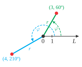
In mathematics, the polar coordinate system is a two-dimensional coordinate system in which each point on a plane is determined by a distance from a reference point and an angle from a reference direction. The reference point is called the pole, and the ray from the pole in the reference direction is the polar axis. The distance from the pole is called the radial coordinate, radial distance or simply radius, and the angle is called the angular coordinate, polar angle, or azimuth. Angles in polar notation are generally expressed in either degrees or radians.
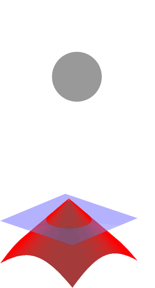
In mathematics, the tangent space of a manifold is a generalization of tangent lines to curves in two-dimensional space and tangent planes to surfaces in three-dimensional space in higher dimensions. In the context of physics the tangent space to a manifold at a point can be viewed as the space of possible velocities for a particle moving on the manifold.

The Navier–Stokes equations are partial differential equations which describe the motion of viscous fluid substances. They were named after French engineer and physicist Claude-Louis Navier and the Irish physicist and mathematician George Gabriel Stokes. They were developed over several decades of progressively building the theories, from 1822 (Navier) to 1842–1850 (Stokes).
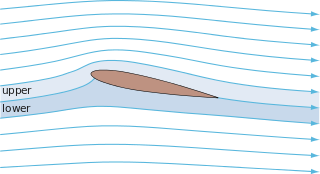
In fluid dynamics, potential flow or irrotational flow refers to a description of a fluid flow with no vorticity in it. Such a description typically arises in the limit of vanishing viscosity, i.e., for an inviscid fluid and with no vorticity present in the flow.

In geometry, a geodesic is a curve representing in some sense the shortest path (arc) between two points in a surface, or more generally in a Riemannian manifold. The term also has meaning in any differentiable manifold with a connection. It is a generalization of the notion of a "straight line".
In vector calculus, Green's theorem relates a line integral around a simple closed curve C to a double integral over the plane region D bounded by C. It is the two-dimensional special case of Stokes' theorem.
Geometrical optics, or ray optics, is a model of optics that describes light propagation in terms of rays. The ray in geometrical optics is an abstraction useful for approximating the paths along which light propagates under certain circumstances.
In mathematics and its applications, the signed distance function is the orthogonal distance of a given point x to the boundary of a set Ω in a metric space, with the sign determined by whether or not x is in the interior of Ω. The function has positive values at points x inside Ω, it decreases in value as x approaches the boundary of Ω where the signed distance function is zero, and it takes negative values outside of Ω. However, the alternative convention is also sometimes taken instead.
In numerical analysis and computational fluid dynamics, Godunov's theorem — also known as Godunov's order barrier theorem — is a mathematical theorem important in the development of the theory of high-resolution schemes for the numerical solution of partial differential equations.
Numerical continuation is a method of computing approximate solutions of a system of parameterized nonlinear equations,
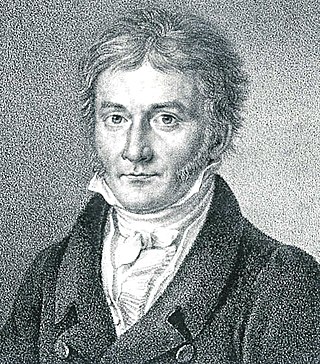
In mathematics, the differential geometry of surfaces deals with the differential geometry of smooth surfaces with various additional structures, most often, a Riemannian metric. Surfaces have been extensively studied from various perspectives: extrinsically, relating to their embedding in Euclidean space and intrinsically, reflecting their properties determined solely by the distance within the surface as measured along curves on the surface. One of the fundamental concepts investigated is the Gaussian curvature, first studied in depth by Carl Friedrich Gauss, who showed that curvature was an intrinsic property of a surface, independent of its isometric embedding in Euclidean space.
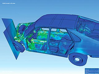
The finite element method (FEM) is a popular method for numerically solving differential equations arising in engineering and mathematical modeling. Typical problem areas of interest include the traditional fields of structural analysis, heat transfer, fluid flow, mass transport, and electromagnetic potential.
In the finite element method for the numerical solution of elliptic partial differential equations, the stiffness matrix is a matrix that represents the system of linear equations that must be solved in order to ascertain an approximate solution to the differential equation.
The Kansa method is a computer method used to solve partial differential equations. Its main advantage is it is very easy to understand and program on a computer. It is much less complicated than the finite element method. Another advantage is it works well on multi variable problems. The finite element method is complicated when working with more than 3 space variables and time.
The power law scheme was first used by Suhas Patankar (1980). It helps in achieving approximate solutions in computational fluid dynamics (CFD) and it is used for giving a more accurate approximation to the one-dimensional exact solution when compared to other schemes in computational fluid dynamics (CFD). This scheme is based on the analytical solution of the convection diffusion equation. This scheme is also very effective in removing False diffusion error.
The hybrid difference scheme is a method used in the numerical solution for convection–diffusion problems. It was introduced by Spalding (1970). It is a combination of central difference scheme and upwind difference scheme as it exploits the favorable properties of both of these schemes.
The Finite volume method in computational fluid dynamics is a discretization technique for partial differential equations that arise from physical conservation laws. These equations can be different in nature, e.g. elliptic, parabolic, or hyperbolic. The first well-documented use of this method was by Evans and Harlow (1957) at Los Alamos. The general equation for steady diffusion can easily be derived from the general transport equation for property Φ by deleting transient and convective terms.
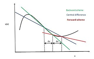
In applied mathematics, the central differencing scheme is a finite difference method that optimizes the approximation for the differential operator in the central node of the considered patch and provides numerical solutions to differential equations. It is one of the schemes used to solve the integrated convection–diffusion equation and to calculate the transported property Φ at the e and w faces, where e and w are short for east and west. The method's advantages are that it is easy to understand and implement, at least for simple material relations; and that its convergence rate is faster than some other finite differencing methods, such as forward and backward differencing. The right side of the convection-diffusion equation, which basically highlights the diffusion terms, can be represented using central difference approximation. To simplify the solution and analysis, linear interpolation can be used logically to compute the cell face values for the left side of this equation, which is nothing but the convective terms. Therefore, cell face values of property for a uniform grid can be written as:
Finite volume method (FVM) is a numerical method. FVM in computational fluid dynamics is used to solve the partial differential equation which arises from the physical conservation law by using discretisation. Convection is always followed by diffusion and hence where convection is considered we have to consider combine effect of convection and diffusion. But in places where fluid flow plays a non-considerable role we can neglect the convective effect of the flow. In this case we have to consider more simplistic case of only diffusion. The general equation for steady convection-diffusion can be easily derived from the general transport equation for property by deleting transient.

The methods used for solving two dimensional Diffusion problems are similar to those used for one dimensional problems. The general equation for steady diffusion can be easily derived from the general transport equation for property Φ by deleting transient and convective terms


