Recursive least squares filter

Last updated

Recursive least squares (RLS) is an adaptive filter algorithm that recursively finds the coefficients that minimize a weighted linear least squares cost function relating to the input signals. This approach is in contrast to other algorithms such as the least mean squares (LMS) that aim to reduce the mean square error. In the derivation of the RLS, the input signals are considered deterministic, while for the LMS and similar algorithms they are considered stochastic. Compared to most of its competitors, the RLS exhibits extremely fast convergence. However, this benefit comes at the cost of high computational complexity.

Contents

Motivation

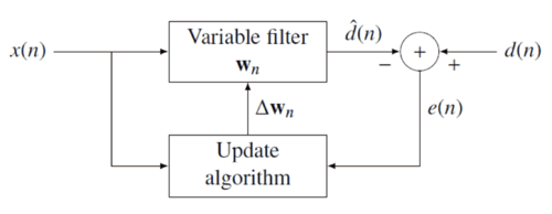
RLS was discovered by Gauss but lay unused or ignored until 1950 when Plackett rediscovered the original work of Gauss from 1821. In general, the RLS can be used to solve any problem that can be solved by adaptive filters. For example, suppose that a signal is transmitted over an echoey, noisy channel that causes it to be received as

where represents additive noise. The intent of the RLS filter is to recover the desired signal by use of a -tap FIR filter, :

where is the column vector containing the most recent samples of . The estimate of the recovered desired signal is

The goal is to estimate the parameters of the filter , and at each time we refer to the current estimate as and the adapted least-squares estimate by . is also a column vector, as shown below, and the transpose, , is a row vector. The matrix product (which is the dot product of and ) is , a scalar. The estimate is "good" if is small in magnitude in some least squares sense.

As time evolves, it is desired to avoid completely redoing the least squares algorithm to find the new estimate for , in terms of .

The benefit of the RLS algorithm is that there is no need to invert matrices, thereby saving computational cost. Another advantage is that it provides intuition behind such results as the Kalman filter.

Discussion

The idea behind RLS filters is to minimize a cost function by appropriately selecting the filter coefficients , updating the filter as new data arrives. The error signal and desired signal are defined in the negative feedback diagram below:

AdaptiveFilter C.png

The error implicitly depends on the filter coefficients through the estimate :

The weighted least squares error function —the cost function we desire to minimize—being a function of is therefore also dependent on the filter coefficients:

where is the "forgetting factor" which gives exponentially less weight to older error samples.

The cost function is minimized by taking the partial derivatives for all entries of the coefficient vector and setting the results to zero

Next, replace with the definition of the error signal

Rearranging the equation yields

This form can be expressed in terms of matrices

where is the weighted sample covariance matrix for , and is the equivalent estimate for the cross-covariance between and . Based on this expression we find the coefficients which minimize the cost function as

This is the main result of the discussion.

Choosing λ

The smaller is, the smaller is the contribution of previous samples to the covariance matrix. This makes the filter more sensitive to recent samples, which means more fluctuations in the filter co-efficients. The case is referred to as the growing window RLS algorithm. In practice, is usually chosen between 0.98 and 1. [1] By using type-II maximum likelihood estimation the optimal can be estimated from a set of data. [2]

Recursive algorithm

The discussion resulted in a single equation to determine a coefficient vector which minimizes the cost function. In this section we want to derive a recursive solution of the form

where is a correction factor at time . We start the derivation of the recursive algorithm by expressing the cross covariance in terms of

where is the dimensional data vector

Similarly we express in terms of by

In order to generate the coefficient vector we are interested in the inverse of the deterministic auto-covariance matrix. For that task the Woodbury matrix identity comes in handy. With

is -by-
is -by-1 (column vector)
is 1-by- (row vector)
is the 1-by-1 identity matrix

The Woodbury matrix identity follows

To come in line with the standard literature, we define

where the gain vector is

Before we move on, it is necessary to bring into another form

Subtracting the second term on the left side yields

With the recursive definition of the desired form follows

Now we are ready to complete the recursion. As discussed

The second step follows from the recursive definition of . Next we incorporate the recursive definition of together with the alternate form of and get

With we arrive at the update equation

where is the a priori error. Compare this with the a posteriori error; the error calculated after the filter is updated:

That means we found the correction factor

This intuitively satisfying result indicates that the correction factor is directly proportional to both the error and the gain vector, which controls how much sensitivity is desired, through the weighting factor, .

RLS algorithm summary

The RLS algorithm for a p-th order RLS filter can be summarized as

Parameters: filter order
forgetting factor
value to initialize
Initialization:,
,
where is the identity matrix of rank
Computation:For

.

The recursion for follows an algebraic Riccati equation and thus draws parallels to the Kalman filter. [3]

Lattice recursive least squares filter (LRLS)

The lattice recursive least squares adaptive filter is related to the standard RLS except that it requires fewer arithmetic operations (order N). [4] It offers additional advantages over conventional LMS algorithms such as faster convergence rates, modular structure, and insensitivity to variations in eigenvalue spread of the input correlation matrix. The LRLS algorithm described is based on a posteriori errors and includes the normalized form. The derivation is similar to the standard RLS algorithm and is based on the definition of . In the forward prediction case, we have with the input signal as the most up to date sample. The backward prediction case is , where i is the index of the sample in the past we want to predict, and the input signal is the most recent sample. [5]

Parameter summary

is the forward reflection coefficient
is the backward reflection coefficient
represents the instantaneous a posteriori forward prediction error
represents the instantaneous a posteriori backward prediction error
is the minimum least-squares backward prediction error
is the minimum least-squares forward prediction error
is a conversion factor between a priori and a posteriori errors
are the feedforward multiplier coefficients.
is a small positive constant that can be 0.01

LRLS algorithm summary

The algorithm for a LRLS filter can be summarized as

Initialization:
For
  (if for )


End
Computation:
For


 For


 Feedforward filtering


 End
End

Normalized lattice recursive least squares filter (NLRLS)

The normalized form of the LRLS has fewer recursions and variables. It can be calculated by applying a normalization to the internal variables of the algorithm which will keep their magnitude bounded by one. This is generally not used in real-time applications because of the number of division and square-root operations which comes with a high computational load.

NLRLS algorithm summary

The algorithm for a NLRLS filter can be summarized as

Initialization:
For
  (if for )
 
 
End
 
Computation:
For
  (Input signal energy)
  (Reference signal energy)
 
 
 For


 Feedforward filter
 
 
 End
End

See also

Related Research Articles

Linear prediction is a mathematical operation where future values of a discrete-time signal are estimated as a linear function of previous samples.

In machine learning, support vector machines are supervised max-margin models with associated learning algorithms that analyze data for classification and regression analysis. Developed at AT&T Bell Laboratories by Vladimir Vapnik with colleagues SVMs are one of the most studied models, being based on statistical learning frameworks of VC theory proposed by Vapnik and Chervonenkis (1974).

<span class="mw-page-title-main">Principal component analysis</span> Method of data analysis

Principal component analysis (PCA) is a linear dimensionality reduction technique with applications in exploratory data analysis, visualization and data preprocessing.

In statistics, the Gauss–Markov theorem states that the ordinary least squares (OLS) estimator has the lowest sampling variance within the class of linear unbiased estimators, if the errors in the linear regression model are uncorrelated, have equal variances and expectation value of zero. The errors do not need to be normal for the theorem to apply, nor do they need to be independent and identically distributed.

An adaptive filter is a system with a linear filter that has a transfer function controlled by variable parameters and a means to adjust those parameters according to an optimization algorithm. Because of the complexity of the optimization algorithms, almost all adaptive filters are digital filters. Adaptive filters are required for some applications because some parameters of the desired processing operation are not known in advance or are changing. The closed loop adaptive filter uses feedback in the form of an error signal to refine its transfer function.

<span class="mw-page-title-main">Kalman filter</span> Algorithm that estimates unknowns from a series of measurements over time

For statistics and control theory, Kalman filtering, also known as linear quadratic estimation (LQE), is an algorithm that uses a series of measurements observed over time, including statistical noise and other inaccuracies, and produces estimates of unknown variables that tend to be more accurate than those based on a single measurement alone, by estimating a joint probability distribution over the variables for each timeframe. The filter is named after Rudolf E. Kálmán, who was one of the primary developers of its theory.

In mathematics, a Hermitian matrix is a complex square matrix that is equal to its own conjugate transpose—that is, the element in the i-th row and j-th column is equal to the complex conjugate of the element in the j-th row and i-th column, for all indices i and j:

In the theory of stochastic processes, the Karhunen–Loève theorem, also known as the Kosambi–Karhunen–Loève theorem states that a stochastic process can be represented as an infinite linear combination of orthogonal functions, analogous to a Fourier series representation of a function on a bounded interval. The transformation is also known as Hotelling transform and eigenvector transform, and is closely related to principal component analysis (PCA) technique widely used in image processing and in data analysis in many fields.

<span class="mw-page-title-main">Gauss–Newton algorithm</span> Mathematical algorithm

The Gauss–Newton algorithm is used to solve non-linear least squares problems, which is equivalent to minimizing a sum of squared function values. It is an extension of Newton's method for finding a minimum of a non-linear function. Since a sum of squares must be nonnegative, the algorithm can be viewed as using Newton's method to iteratively approximate zeroes of the components of the sum, and thus minimizing the sum. In this sense, the algorithm is also an effective method for solving overdetermined systems of equations. It has the advantage that second derivatives, which can be challenging to compute, are not required.

In signal processing, the Wiener filter is a filter used to produce an estimate of a desired or target random process by linear time-invariant (LTI) filtering of an observed noisy process, assuming known stationary signal and noise spectra, and additive noise. The Wiener filter minimizes the mean square error between the estimated random process and the desired process.

<span class="mw-page-title-main">Adaptive equalizer</span>

An adaptive equalizer is an equalizer that automatically adapts to time-varying properties of the communication channel. It is frequently used with coherent modulations such as phase-shift keying, mitigating the effects of multipath propagation and Doppler spreading.

Least mean squares (LMS) algorithms are a class of adaptive filter used to mimic a desired filter by finding the filter coefficients that relate to producing the least mean square of the error signal. It is a stochastic gradient descent method in that the filter is only adapted based on the error at the current time. It was invented in 1960 by Stanford University professor Bernard Widrow and his first Ph.D. student, Ted Hoff, based on their research in single-layer neural networks (ADALINE). Specifically, they used gradient descent to train ADALINE to recognize patterns, and called the algorithm "delta rule". They then applied the rule to filters, resulting in the LMS algorithm.

In linear algebra, it is often important to know which vectors have their directions unchanged by a given linear transformation. An eigenvector or characteristic vector is such a vector. Thus an eigenvector of a linear transformation is scaled by a constant factor when the linear transformation is applied to it: . The corresponding eigenvalue, characteristic value, or characteristic root is the multiplying factor .

In linear algebra, a frame of an inner product space is a generalization of a basis of a vector space to sets that may be linearly dependent. In the terminology of signal processing, a frame provides a redundant, stable way of representing a signal. Frames are used in error detection and correction and the design and analysis of filter banks and more generally in applied mathematics, computer science, and engineering.

In linear algebra, eigendecomposition is the factorization of a matrix into a canonical form, whereby the matrix is represented in terms of its eigenvalues and eigenvectors. Only diagonalizable matrices can be factorized in this way. When the matrix being factorized is a normal or real symmetric matrix, the decomposition is called "spectral decomposition", derived from the spectral theorem.

Non-linear least squares is the form of least squares analysis used to fit a set of m observations with a model that is non-linear in n unknown parameters (m ≥ n). It is used in some forms of nonlinear regression. The basis of the method is to approximate the model by a linear one and to refine the parameters by successive iterations. There are many similarities to linear least squares, but also some significant differences. In economic theory, the non-linear least squares method is applied in (i) the probit regression, (ii) threshold regression, (iii) smooth regression, (iv) logistic link regression, (v) Box–Cox transformed regressors ().

<span class="mw-page-title-main">Generalized chi-squared distribution</span>

In probability theory and statistics, the generalized chi-squared distribution is the distribution of a quadratic form of a multinormal variable, or a linear combination of different normal variables and squares of normal variables. Equivalently, it is also a linear sum of independent noncentral chi-square variables and a normal variable. There are several other such generalizations for which the same term is sometimes used; some of them are special cases of the family discussed here, for example the gamma distribution.

A two-dimensional (2D) adaptive filter is very much like a one-dimensional adaptive filter in that it is a linear system whose parameters are adaptively updated throughout the process, according to some optimization approach. The main difference between 1D and 2D adaptive filters is that the former usually take as inputs signals with respect to time, what implies in causality constraints, while the latter handles signals with 2 dimensions, like x-y coordinates in the space domain, which are usually non-causal. Moreover, just like 1D filters, most 2D adaptive filters are digital filters, because of the complex and iterative nature of the algorithms.

Regularized least squares (RLS) is a family of methods for solving the least-squares problem while using regularization to further constrain the resulting solution.

Sparse dictionary learning is a representation learning method which aims at finding a sparse representation of the input data in the form of a linear combination of basic elements as well as those basic elements themselves. These elements are called atoms and they compose a dictionary. Atoms in the dictionary are not required to be orthogonal, and they may be an over-complete spanning set. This problem setup also allows the dimensionality of the signals being represented to be higher than the one of the signals being observed. The above two properties lead to having seemingly redundant atoms that allow multiple representations of the same signal but also provide an improvement in sparsity and flexibility of the representation.

References

Notes

  1. Emannual C. Ifeacor, Barrie W. Jervis. Digital signal processing: a practical approach, second edition. Indianapolis: Pearson Education Limited, 2002, p. 718
  2. Steven Van Vaerenbergh, Ignacio Santamaría, Miguel Lázaro-Gredilla "Estimation of the forgetting factor in kernel recursive least squares", 2012 IEEE International Workshop on Machine Learning for Signal Processing, 2012, accessed June 23, 2016.
  3. Welch, Greg and Bishop, Gary "An Introduction to the Kalman Filter", Department of Computer Science, University of North Carolina at Chapel Hill, September 17, 1997, accessed July 19, 2011.
  4. Diniz, Paulo S.R., "Adaptive Filtering: Algorithms and Practical Implementation", Springer Nature Switzerland AG 2020, Chapter 7: Adaptive Lattice-Based RLS Algorithms. https://doi.org/10.1007/978-3-030-29057-3_7
  5. Albu, Kadlec, Softley, Matousek, Hermanek, Coleman, Fagan "Implementation of (Normalised) RLS Lattice on Virtex", Digital Signal Processing, 2001, accessed December 24, 2011.