In fluid dynamics, turbulence or turbulent flow is fluid motion characterized by chaotic changes in pressure and flow velocity. It is in contrast to a laminar flow, which occurs when a fluid flows in parallel layers, with no disruption between those layers.
The Richardson number (Ri) is named after Lewis Fry Richardson (1881–1953). It is the dimensionless number that expresses the ratio of the buoyancy term to the flow shear term:

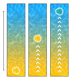
Internal waves are gravity waves that oscillate within a fluid medium, rather than on its surface. To exist, the fluid must be stratified: the density must change with depth/height due to changes, for example, in temperature and/or salinity. If the density changes over a small vertical distance, the waves propagate horizontally like surface waves, but do so at slower speeds as determined by the density difference of the fluid below and above the interface. If the density changes continuously, the waves can propagate vertically as well as horizontally through the fluid.

In meteorology, the planetary boundary layer (PBL), also known as the atmospheric boundary layer (ABL) or peplosphere, is the lowest part of the atmosphere and its behaviour is directly influenced by its contact with a planetary surface. On Earth it usually responds to changes in surface radiative forcing in an hour or less. In this layer physical quantities such as flow velocity, temperature, and moisture display rapid fluctuations (turbulence) and vertical mixing is strong. Above the PBL is the "free atmosphere", where the wind is approximately geostrophic, while within the PBL the wind is affected by surface drag and turns across the isobars.

A pycnocline is the cline or layer where the density gradient is greatest within a body of water. An ocean current is generated by the forces such as breaking waves, temperature and salinity differences, wind, Coriolis effect, and tides caused by the gravitational pull of the Moon and the Sun. In addition, the physical properties in a pycnocline driven by density gradients also affect the flows and vertical profiles in the ocean. These changes can be connected to the transport of heat, salt, and nutrients through the ocean, and the pycnocline diffusion controls upwelling.
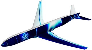
Turbulence modeling is the construction and use of a mathematical model to predict the effects of turbulence. Turbulent flows are commonplace in most real life scenarios, including the flow of blood through the cardiovascular system, the airflow over an aircraft wing, the re-entry of space vehicles, besides others. In spite of decades of research, there is no analytical theory to predict the evolution of these turbulent flows. The equations governing turbulent flows can only be solved directly for simple cases of flow. For most real life turbulent flows, CFD simulations use turbulent models to predict the evolution of turbulence. These turbulence models are simplified constitutive equations that predict the statistical evolution of turbulent flows.

In fluid dynamics, an eddy is the swirling of a fluid and the reverse current created when the fluid is in a turbulent flow regime. The moving fluid creates a space devoid of downstream-flowing fluid on the downstream side of the object. Fluid behind the obstacle flows into the void creating a swirl of fluid on each edge of the obstacle, followed by a short reverse flow of fluid behind the obstacle flowing upstream, toward the back of the obstacle. This phenomenon is naturally observed behind large emergent rocks in swift-flowing rivers.

The Ekman layer is the layer in a fluid where there is a force balance between pressure gradient force, Coriolis force and turbulent drag. It was first described by Vagn Walfrid Ekman. Ekman layers occur both in the atmosphere and in the ocean.
Stratification is defined as the separation of water in layers based on a specific quantity. Two main types of stratification of water are uniform and layered stratification. Layered stratification occurs in all of the ocean basins. The stratified layers act as a barrier to the mixing of water, which can impact the exchange of heat, carbon, oxygen and other nutrients. Due to upwelling and downwelling, which are both wind-driven, mixing of different layers can occur by means of the rise of cold nutrient-rich and warm water, respectively. Generally, the layers are based on the density of water. Intuitively, heavier, and hence denser, water is located below the lighter water, representing a stable stratification. An example of a layer in the ocean is the pycnocline, which is defined as a layer in the ocean where the change in density is relatively large compared to the other layers in the ocean. The thickness of the thermocline is not constant everywhere, but depends on a variety of variables. Over the years stratification of the ocean basins has increased. An increase in stratification means that the differences in density of the layers in the oceans increase, leading to for example larger mixing barriers.
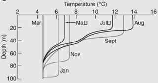
The oceanic or limnological mixed layer is a layer in which active turbulence has homogenized some range of depths. The surface mixed layer is a layer where this turbulence is generated by winds, surface heat fluxes, or processes such as evaporation or sea ice formation which result in an increase in salinity. The atmospheric mixed layer is a zone having nearly constant potential temperature and specific humidity with height. The depth of the atmospheric mixed layer is known as the mixing height. Turbulence typically plays a role in the formation of fluid mixed layers.
In fluid dynamics, turbulence kinetic energy (TKE) is the mean kinetic energy per unit mass associated with eddies in turbulent flow. Physically, the turbulence kinetic energy is characterised by measured root-mean-square (RMS) velocity fluctuations. In the Reynolds-averaged Navier Stokes equations, the turbulence kinetic energy can be calculated based on the closure method, i.e. a turbulence model.
The Obukhov length is used to describe the effects of buoyancy on turbulent flows, particularly in the lower tenth of the atmospheric boundary layer. It was first defined by Alexander Obukhov in 1946. It is also known as the Monin–Obukhov length because of its important role in the similarity theory developed by Monin and Obukhov. A simple definition of the Monin-Obukhov length is that height at which turbulence is generated more by buoyancy than by wind shear.
Ekman transport is part of Ekman motion theory, first investigated in 1902 by Vagn Walfrid Ekman. Winds are the main source of energy for ocean circulation, and Ekman Transport is a component of wind-driven ocean current. Ekman transport occurs when ocean surface waters are influenced by the friction force acting on them via the wind. As the wind blows it casts a friction force on the ocean surface that drags the upper 10-100m of the water column with it. However, due to the influence of the Coriolis effect, the ocean water moves at a 90° angle from the direction of the surface wind. The direction of transport is dependent on the hemisphere: in the northern hemisphere, transport occurs at 90° clockwise from wind direction, while in the southern hemisphere it occurs at 90° anticlockwise. This phenomenon was first noted by Fridtjof Nansen, who recorded that ice transport appeared to occur at an angle to the wind direction during his Arctic expedition during the 1890s. Ekman transport has significant impacts on the biogeochemical properties of the world's oceans. This is because it leads to upwelling and downwelling in order to obey mass conservation laws. Mass conservation, in reference to Ekman transfer, requires that any water displaced within an area must be replenished. This can be done by either Ekman suction or Ekman pumping depending on wind patterns.
For a pure wave motion in fluid dynamics, the Stokes drift velocity is the average velocity when following a specific fluid parcel as it travels with the fluid flow. For instance, a particle floating at the free surface of water waves, experiences a net Stokes drift velocity in the direction of wave propagation.
Ocean dynamics define and describe the motion of water within the oceans. Ocean temperature and motion fields can be separated into three distinct layers: mixed (surface) layer, upper ocean, and deep ocean.
In fluid dynamics, the mixing length model is a method attempting to describe momentum transfer by turbulence Reynolds stresses within a Newtonian fluid boundary layer by means of an eddy viscosity. The model was developed by Ludwig Prandtl in the early 20th century. Prandtl himself had reservations about the model, describing it as, "only a rough approximation," but it has been used in numerous fields ever since, including atmospheric science, oceanography and stellar structure.
In oceanography, Ekman velocity – also referred as a kind of the residual ageostropic velocity as it derivates from geostrophy – is part of the total horizontal velocity (u) in the upper layer of water of the open ocean. This velocity, caused by winds blowing over the surface of the ocean, is such that the Coriolis force on this layer is balanced by the force of the wind.
The convective planetary boundary layer (CPBL), also known as the daytime planetary boundary layer, is the part of the lower troposphere most directly affected by solar heating of the earth's surface.
Open ocean convection is a process in which the mesoscale ocean circulation and large, strong winds mix layers of water at different depths. Fresher water lying over the saltier or warmer over the colder leads to the stratification of water, or its separation into layers. Strong winds cause evaporation, so the ocean surface cools, weakening the stratification. As a result, the surface waters are overturned and sink while the "warmer" waters rise to the surface, starting the process of convection. This process has a crucial role in the formation of both bottom and intermediate water and in the large-scale thermohaline circulation, which largely determines global climate. It is also an important phenomena that controls the intensity of the Atlantic Meridional Overturning Circulation (AMOC).
A baroclinic instability is a fluid dynamical instability of fundamental importance in the atmosphere and ocean. It can lead to the formation of transient mesoscale eddies, with a horizontal scale of 10-100 km. In contrast, flows on the largest scale in the ocean are described as ocean currents, the largest scale eddies are mostly created by shearing of two ocean currents and static mesoscale eddies are formed by the flow around an obstacle (as seen in the animation on eddy. Mesoscale eddies are circular currents with swirling motion and account for approximately 90% of the ocean's total kinetic energy. Therefore, they are key in mixing and transport of for example heat, salt and nutrients.


