Almost periodic function

Not to be confused with Quasiperiodic function.

In mathematics, an almost periodic function is, loosely speaking, a function of a real number that is periodic to within any desired level of accuracy, given suitably long, well-distributed "almost-periods". The concept was first studied by Harald Bohr and later generalized by Vyacheslav Stepanov, Hermann Weyl and Abram Samoilovitch Besicovitch, amongst others. There is also a notion of almost periodic functions on locally compact abelian groups, first studied by John von Neumann.

Almost periodicity is a property of dynamical systems that appear to retrace their paths through phase space, but not exactly. An example would be a planetary system, with planets in orbits moving with periods that are not commensurable (i.e., with a period vector that is not proportional to a vector of integers). A theorem of Kronecker from diophantine approximation can be used to show that any particular configuration that occurs once, will recur to within any specified accuracy: if we wait long enough we can observe the planets all return to within a second of arc to the positions they once were in.

Motivation

There are several inequivalent definitions of almost periodic functions. The first was given by Harald Bohr. His interest was initially in finite Dirichlet series. In fact by truncating the series for the Riemann zeta function ζ(s) to make it finite, one gets finite sums of terms of the type

${\displaystyle e^{s\log n}\,}$

with s written as (σ + it) – the sum of its real part σ and imaginary part it. Fixing σ, so restricting attention to a single vertical line in the complex plane, we can see this also as

${\displaystyle n^{\sigma }e^{(\log n)it}.\,}$

Taking a finite sum of such terms avoids difficulties of analytic continuation to the region σ < 1. Here the 'frequencies' log n will not all be commensurable (they are as linearly independent over the rational numbers as the integers n are multiplicatively independent – which comes down to their prime factorizations).

With this initial motivation to consider types of trigonometric polynomial with independent frequencies, mathematical analysis was applied to discuss the closure of this set of basic functions, in various norms.

The theory was developed using other norms by Besicovitch, Stepanov, Weyl, von Neumann, Turing, Bochner and others in the 1920s and 1930s.

Uniform or Bohr or Bochner almost periodic functions

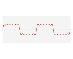
Bohr (1925) ^[1] defined the uniformly almost-periodic functions as the closure of the trigonometric polynomials with respect to the uniform norm

${\displaystyle \|f\|_{\infty }=\sup _{x}|f(x)|}$

(on bounded functions f on R). In other words, a function f is uniformly almost periodic if for every ε > 0 there is a finite linear combination of sine and cosine waves that is of distance less than ε from f with respect to the uniform norm. The sine and cosine frequencies can be arbitrary real numbers. Bohr proved that this definition was equivalent to the existence of a relatively dense set of ε almost-periods, for all ε > 0: that is, translations T(ε) = T of the variable t making

${\displaystyle \left|f(t+T)-f(t)\right|<\varepsilon .}$

An alternative definition due to Bochner (1926) is equivalent to that of Bohr and is relatively simple to state:

A function f is almost periodic if every sequence {ƒ(t + T_n)} of translations of f has a subsequence that converges uniformly for t in (−∞, +∞).

The Bohr almost periodic functions are essentially the same as continuous functions on the Bohr compactification of the reals.

Stepanov almost periodic functions

The space S^p of Stepanov almost periodic functions (for p ≥ 1) was introduced by V.V. Stepanov (1925). ^[2] It contains the space of Bohr almost periodic functions. It is the closure of the trigonometric polynomials under the norm

${\displaystyle \|f\|_{S,r,p}=\sup _{x}\left({1 \over r}\int _{x}^{x+r}|f(s)|^{p}\,ds\right)^{1/p}}$

for any fixed positive value of r; for different values of r these norms give the same topology and so the same space of almost periodic functions (though the norm on this space depends on the choice of r).

Weyl almost periodic functions

The space W^p of Weyl almost periodic functions (for p ≥ 1) was introduced by Weyl (1927). ^[3] It contains the space S^p of Stepanov almost periodic functions. It is the closure of the trigonometric polynomials under the seminorm

${\displaystyle \|f\|_{W,p}=\lim _{r\to \infty }\|f\|_{S,r,p}}$

Warning: there are nonzero functions ƒ with ||ƒ||_W,p = 0, such as any bounded function of compact support, so to get a Banach space one has to quotient out by these functions.

Besicovitch almost periodic functions

The space B^p of Besicovitch almost periodic functions was introduced by Besicovitch (1926). ^[4] It is the closure of the trigonometric polynomials under the seminorm

${\displaystyle \|f\|_{B,p}=\limsup _{x\to \infty }\left({1 \over 2x}\int _{-x}^{x}|f(s)|^{p}\,ds\right)^{1/p}}$

Warning: there are nonzero functions ƒ with ||ƒ||_B,p = 0, such as any bounded function of compact support, so to get a Banach space one has to quotient out by these functions.

The Besicovitch almost periodic functions in B² have an expansion (not necessarily convergent) as

${\displaystyle \sum a_{n}e^{i\lambda _{n}t}}$

with Σa²
_n finite and λ_n real. Conversely every such series is the expansion of some Besicovitch periodic function (which is not unique).

The space B^p of Besicovitch almost periodic functions (for p ≥ 1) contains the space W^p of Weyl almost periodic functions. If one quotients out a subspace of "null" functions, it can be identified with the space of L^p functions on the Bohr compactification of the reals.

Almost periodic functions on a locally compact group

With these theoretical developments and the advent of abstract methods (the Peter–Weyl theorem, Pontryagin duality and Banach algebras) a general theory became possible. The general idea of almost-periodicity in relation to a locally compact abelian group G becomes that of a function F in L^∞(G), such that its translates by G form a relatively compact set. Equivalently, the space of almost periodic functions is the norm closure of the finite linear combinations of characters of G. If G is compact the almost periodic functions are the same as the continuous functions.

The Bohr compactification of G is the compact abelian group of all possibly discontinuous characters of the dual group of G, and is a compact group containing G as a dense subgroup. The space of uniform almost periodic functions on G can be identified with the space of all continuous functions on the Bohr compactification of G. More generally the Bohr compactification can be defined for any topological group G, and the spaces of continuous or L^p functions on the Bohr compactification can be considered as almost periodic functions on G. For locally compact connected groups G the map from G to its Bohr compactification is injective if and only if G is a central extension of a compact group, or equivalently the product of a compact group and a finite-dimensional vector space.

A function on a locally compact group is called weakly almost periodic if its orbit is weakly relatively compact in ${\displaystyle L^{\infty }}$.

Given a topological dynamical system ${\displaystyle (X,G)}$ consisting of a compact topological space X with an action of the locally compact group G, a continuous function on X is (weakly) almost periodic if its orbit is (weakly) precompact in the Banach space ${\displaystyle C(X)}$.

Quasiperiodic signals in audio and music synthesis

In speech processing, audio signal processing, and music synthesis, a quasiperiodic signal, sometimes called a quasiharmonic signal, is a waveform that is virtually periodic microscopically, but not necessarily periodic macroscopically. This does not give a quasiperiodic function in the sense of the Wikipedia article of that name, but something more akin to an almost periodic function, being a nearly periodic function where any one period is virtually identical to its adjacent periods but not necessarily similar to periods much farther away in time. This is the case for musical tones (after the initial attack transient) where all partials or overtones are harmonic (that is all overtones are at frequencies that are an integer multiple of a fundamental frequency of the tone).

When a signal ${\displaystyle x(t)\ }$ is fully periodic with period ${\displaystyle P\ }$, then the signal exactly satisfies

${\displaystyle x(t)=x(t+P)\qquad \forall t\in \mathbb {R} }$

or

${\displaystyle {\Big |}x(t)-x(t+P){\Big |}=0\qquad \forall t\in \mathbb {R} .\ }$

The Fourier series representation would be

${\displaystyle x(t)=a_{0}+\sum _{n=1}^{\infty }{\big [}a_{n}\cos(2\pi nf_{0}t)-b_{n}\sin(2\pi nf_{0}t){\big ]}}$

or

${\displaystyle x(t)=a_{0}+\sum _{n=1}^{\infty }r_{n}\cos(2\pi nf_{0}t+\varphi _{n})}$

where ${\displaystyle f_{0}={\frac {1}{P}}}$ is the fundamental frequency and the Fourier coefficients are

${\displaystyle a_{0}={\frac {1}{P}}\int _{t_{0}}^{t_{0}+P}x(t)\,dt\ }$

${\displaystyle a_{n}=r_{n}\cos \left(\varphi _{n}\right)={\frac {2}{P}}\int _{t_{0}}^{t_{0}+P}x(t)\cos(2\pi nf_{0}t)\,dt\qquad n\geq 1}$

${\displaystyle b_{n}=r_{n}\sin \left(\varphi _{n}\right)=-{\frac {2}{P}}\int _{t_{0}}^{t_{0}+P}x(t)\sin(2\pi nf_{0}t)\,dt\ }$

where ${\displaystyle t_{0}\ }$ can be any time: ${\displaystyle -\infty <t_{0}<+\infty \ }$.

The fundamental frequency ${\displaystyle f_{0}\ }$, and Fourier coefficients ${\displaystyle a_{n}\ }$, ${\displaystyle b_{n}\ }$, ${\displaystyle r_{n}\ }$, or ${\displaystyle \varphi _{n}\ }$, are constants, i.e. they are not functions of time. The harmonic frequencies are exact integer multiples of the fundamental frequency.

When ${\displaystyle x(t)\ }$ is quasiperiodic then

${\displaystyle x(t)\approx x{\big (}t+P(t){\big )}\ }$

or

${\displaystyle {\Big |}x(t)-x{\big (}t+P(t){\big )}{\Big |}<\varepsilon \ }$

where

${\displaystyle 0<\epsilon \ll {\big \Vert }x{\big \Vert }={\sqrt {\overline {x^{2}}}}={\sqrt {\lim _{\tau \to \infty }{\frac {1}{\tau }}\int _{-\tau /2}^{\tau /2}x^{2}(t)\,dt}}.\ }$

Now the Fourier series representation would be

${\displaystyle x(t)=a_{0}(t)\ +\ \sum _{n=1}^{\infty }\left[a_{n}(t)\cos \left(2\pi n\int _{0}^{t}f_{0}(\tau )\,d\tau \right)-b_{n}(t)\sin \left(2\pi n\int _{0}^{t}f_{0}(\tau )\,d\tau \right)\right]}$

or

${\displaystyle x(t)=a_{0}(t)\ +\ \sum _{n=1}^{\infty }r_{n}(t)\cos \left(2\pi n\int _{0}^{t}f_{0}(\tau )\,d\tau +\varphi _{n}(t)\right)}$

or

${\displaystyle x(t)=a_{0}(t)+\sum _{n=1}^{\infty }r_{n}(t)\cos \left(2\pi \int _{0}^{t}f_{n}(\tau )\,d\tau +\varphi _{n}(0)\right)}$

where ${\displaystyle f_{0}(t)={\frac {1}{P(t)}}}$ is the possibly time-varying fundamental frequency and the time-varying Fourier coefficients are

${\displaystyle a_{0}(t)={\frac {1}{P(t)}}\int _{t-P(t)/2}^{t+P(t)/2}x(\tau )\,d\tau \ }$

${\displaystyle a_{n}(t)=r_{n}(t)\cos {\big (}\varphi _{n}(t){\big )}={\frac {2}{P(t)}}\int _{t-P(t)/2}^{t+P(t)/2}x(\tau )\cos {\big (}2\pi nf_{0}(t)\tau {\big )}\,d\tau \qquad n\geq 1}$

${\displaystyle b_{n}(t)=r_{n}(t)\sin {\big (}\varphi _{n}(t){\big )}=-{\frac {2}{P(t)}}\int _{t-P(t)/2}^{t+P(t)/2}x(\tau )\sin {\big (}2\pi nf_{0}(t)\tau {\big )}\,d\tau \ }$

and the instantaneous frequency for each partial is

${\displaystyle f_{n}(t)=nf_{0}(t)+{\frac {1}{2\pi }}\varphi _{n}^{\prime }(t).\,}$

Whereas in this quasiperiodic case, the fundamental frequency ${\displaystyle f_{0}(t)\ }$, the harmonic frequencies ${\displaystyle f_{n}(t)\ }$, and the Fourier coefficients ${\displaystyle a_{n}(t)\ }$, ${\displaystyle b_{n}(t)\ }$, ${\displaystyle r_{n}(t)\ }$, or ${\displaystyle \varphi _{n}(t)\ }$ are not necessarily constant, and are functions of time albeit slowly varying functions of time. Stated differently these functions of time are bandlimited to much less than the fundamental frequency for ${\displaystyle x(t)\ }$ to be considered to be quasiperiodic.

The partial frequencies ${\displaystyle f_{n}(t)\ }$ are very nearly harmonic but not necessarily exactly so. The time-derivative of ${\displaystyle \varphi _{n}(t)\ }$, that is ${\displaystyle \varphi _{n}^{\prime }(t)\ }$, has the effect of detuning the partials from their exact integer harmonic value ${\displaystyle nf_{0}(t)\ }$. A rapidly changing ${\displaystyle \varphi _{n}(t)\ }$ means that the instantaneous frequency for that partial is severely detuned from the integer harmonic value which would mean that ${\displaystyle x(t)\ }$ is not quasiperiodic.

See also

• Quasiperiodic function
• Aperiodic function
• Quasiperiodic tiling
• Fourier series
• Additive synthesis
• Harmonic series (music)
• Computer music

References

1. H. Bohr, "Zur Theorie der fastperiodischen Funktionen I" Acta Math., 45 (1925) pp. 29–127
2. W. Stepanoff(=V.V. Stepanov), "Sur quelques généralisations des fonctions presque périodiques" C. R. Acad. Sci. Paris, 181 (1925) pp. 90–92; W. Stepanoff(=V.V. Stepanov), "Ueber einige Verallgemeinerungen der fastperiodischen Funktionen" Math. Ann., 45 (1925) pp. 473–498
3. H. Weyl, "Integralgleichungen und fastperiodische Funktionen" Math. Ann., 97 (1927) pp. 338–356
4. A.S. Besicovitch, "On generalized almost periodic functions" Proc. London Math. Soc. (2), 25 (1926) pp. 495–512

Bibliography

• Amerio, Luigi; Prouse, Giovanni (1971), Almost-periodic functions and functional equations, The University Series in Higher Mathematics, New York–Cincinnati–Toronto–London–Melbourne: Van Nostrand Reinhold, pp. viii+184, ISBN   0-442-20295-4, MR   0275061, Zbl   0215.15701 .
• A.S. Besicovitch, "Almost periodic functions", Cambridge Univ. Press (1932)
• Bochner, S. (1926), "Beitrage zur Theorie der fastperiodischen Funktionen", Math. Annalen, 96: 119–147, doi:10.1007/BF01209156, S2CID   118124462
• S. Bochner and J. von Neumann, "Almost Periodic Function in a Group II", Trans. Amer. Math. Soc., 37 no. 1 (1935) pp. 21–50
• H. Bohr, "Almost-periodic functions", Chelsea, reprint (1947)
• Bredikhina, E.A. (2001) [1994], "Almost-periodic functions", Encyclopedia of Mathematics , EMS Press
• Bredikhina, E.A. (2001) [1994], "Besicovitch almost periodic functions", Encyclopedia of Mathematics , EMS Press
• Bredikhina, E.A. (2001) [1994], "Bohr almost periodic functions", Encyclopedia of Mathematics , EMS Press
• Bredikhina, E.A. (2001) [1994], "Stepanov almost periodic functions", Encyclopedia of Mathematics , EMS Press
• Bredikhina, E.A. (2001) [1994], "Weyl almost periodic functions", Encyclopedia of Mathematics , EMS Press
• J. von Neumann, "Almost Periodic Functions in a Group I", Trans. Amer. Math. Soc., 36 no. 3 (1934) pp. 445–492

External links

• "Almost periodic function (equivalent definition)". PlanetMath .