Balanced flow

Last updated

In atmospheric science, balanced flow is an idealisation of atmospheric motion. The idealisation consists in considering the behaviour of one isolated parcel of air having constant density, its motion on a horizontal plane subject to selected forces acting on it and, finally, steady-state conditions.

Contents

Balanced flow is often an accurate approximation of the actual flow, and is useful in improving the qualitative understanding and interpretation of atmospheric motion. In particular, the balanced-flow speeds can be used as estimates of the wind speed for particular arrangements of the atmospheric pressure on Earth's surface.

The Momentum Equations in Natural Coordinates

Trajectories

The momentum equations are written primarily for the generic trajectory of a packet of flow travelling on a horizontal plane and taken at a certain elapsed time called t. The position of the packet is defined by the distance on the trajectory s=s(t) which it has travelled by time t. In reality, however, the trajectory is the outcome of the balance of forces upon the particle. In this section we assume to know it from the start for convenience of representation. When we consider the motion determined by the forces selected next, we will have clues of which type of trajectory fits the particular balance of forces.

The trajectory at a position s has one tangent unit vector s that invariably points in the direction of growing s's, as well as one unit vector n, perpendicular to s, that points towards the local centre of curvature O. The centre of curvature is found on the 'inner side' of the bend, and can shift across either side of the trajectory according to the shape of it. The distance between the parcel position and the centre of curvature is the radius of curvature R at that position. The radius of curvature approaches an infinite length at the points where the trajectory becomes straight and the positive orientation of n is not determined in this particular case (discussed in geostrophic flows). The frame of reference (s,n) is shown by the red arrows in the figure. This frame is termed natural or intrinsic because the axes continuously adjust to the moving parcel, and so they are the most closely connected to its fate.

Trajectory.jpg

Kinematics

The velocity vector (V) is oriented like s and has intensity (speed) V = ds/dt. This speed is always a positive quantity, since any parcel moves along its own trajectory and, for increasing times (dt>0), the trodden length increases as well (ds>0).

The acceleration vector of the parcel is decomposed in the tangential acceleration parallel to s and in the centripetal acceleration along positive n. The tangential acceleration only changes the speed V and is equal to DV/Dt, where big d's denote the material derivative. The centripetal acceleration always points towards the centre of curvature O and only changes the direction s of the forward displacement while the parcel moves on.

Forces

In the balanced-flow idealization we consider a three-way balance of forces that are:

In the fictitious situation drawn in the figure, the pressure force pushes the parcel forward along the trajectory and inward with respect to the bend; the Coriolis force pushes inwards (outwards) of the bend in the northern (southern) hemisphere; and friction pulls (necessarily) rearwards.

Governing equations

For the dynamical equilibrium of the parcel, either component of acceleration times the parcel's mass is equal to the components of the external forces acting in the same direction. As the equations of equilibrium for the parcel are written in natural coordinates, the component equations for the horizontal momentum per unit mass are expressed as follows:

in the forward and sideway directions respectively, where ρ is the density of air.

The terms can be broken down as follows:

Steady-state assumption

In the following discussions, we consider steady-state flow. The speed cannot thus change with time, and the component forces producing tangential acceleration need to sum up to zero. In other words, active and resistive forces must balance out in the forward direction in order that . Importantly, no assumption is made yet on whether the right-hand side forces are of either significant or negligible magnitude there. Moreover, trajectories and streamlines coincide in steady-state conditions, and the pairs of adjectives tangential/normal and streamwise/cross-stream become interchangeable. An atmospheric flow in which the tangential acceleration is not negligible is called allisobaric.

The velocity direction can still change in space along the trajectory that, excluding inertial flows, is set by the pressure pattern.

General framework

The schematisations

Omitting specific terms in the tangential and normal balance equations, we obtain one of the five following idealized flows: antitriptic, geostrophic, cyclostrophic, inertial, and gradient flows. By reasoning on the balance of the remaining terms, we can understand

The following yes/no table shows which contributions are considered in each idealisation. The Ekman layer's schematisation is also mentioned for completeness, and is treated separately since it involves the internal friction of air rather than that between air and ground.

Antitriptic flow Geostrophic flow Cyclostrophic flow Inertial flow Gradient flow Ekman flow
curvatureNNYYYN
frictionYNNNNY
pressureYYYNYY
CoriolisNYNYYY

The limitations

Vertical differences of air properties

The equations were said to apply to parcels of air moving on horizontal planes. Indeed, when one considers a column of atmosphere, it is seldom the case that the air density is the same all the height up, since temperature and moisture content, hence density, do change with height. Every parcel within such a column moves according to the air properties at its own height.

Homogeneous sheets of air may slide one over the other, so long as stable stratification of lighter air on top of heavier air leads to well-separated layers. If some air happens to be heavier/lighter than that in the surroundings, though, vertical motions do occur and modify the horizontal motion in turn. In nature downdrafts and updrafts can sometimes be more rapid and intense than the motion parallel to the ground. The balanced-flow equations do not contain either a force representing the sinking/buoyancy action or the vertical component of velocity.

Consider also that the pressure is normally known through instruments (barometers) near the ground/sea level. The isobars of the ordinary weather charts summarise these pressure measurements, adjusted to the mean sea level for uniformity of presentation, at one particular time. Such values represent the weight of the air column overhead without indicating the details of the changes of the air's specific weight overhead. Also, by Bernoulli's theorem, the measured pressure is not exactly the weight of the air column, should significant vertical motion of air occur. Thus, the pressure force acting on individual parcels of air at different heights is not really known through the measured values. When using information from a surface-pressure chart in balanced-flow formulations, the forces are best viewed as applied to the entire air column.

One difference of air speed in every air column invariably occurs, however, near the ground/sea, also if the air density is the same anywhere and no vertical motion occurs. There, the roughness of the contact surface slows down the air motion above, and this retarding effect peters out with height. See, for example, planetary boundary layer. Frictional antitriptic flow applies near the ground, while the other schematisations apply far enough from the ground not to feel its "braking" effect (free-air flow). This is a reason to keep the two groups conceptually separated. The transition from low-quote to high-quote schematisations is bridged by Ekman-like schematisations where air-to-air friction, Coriolis and pressure forces are in balance.

In summary, the balanced-flow speeds apply well to air columns that can be regarded as homogeneous (constant density, no vertical motion) or, at most, stably stratified (non-constant density, yet no vertical motion). An uncertainty in the estimate arises if we are not able to verify these conditions to occur. They also cannot describe the motion of the entire column from the contact surface with the Earth up to the outer atmosphere, because of the on-off handling of the friction forces.

Horizontal differences of air properties

Even if air columns are homogeneous with height, the density of each column can change from location to location, firstly since air masses have different temperatures and moisture content depending on their origin; and then since air masses modify their properties as they flow over Earth's surface. For example, in extra-tropical cyclones the air circulating around a pressure low typically comes with a sector of warmer temperature wedged within colder air. The gradient-flow model of cyclonic circulation does not allow for these features.

Balanced-flow schematisations can be used to estimate the wind speed in air flows covering several degrees of latitude of Earth's surface. However, in this case assuming a constant Coriolis parameter is unrealistic, and the balanced-flow speed can be applied locally. See Rossby waves as an example of when changes of latitude are dynamically effective.

Unsteadiness

The balanced-flow approach identifies typical trajectories and steady-state wind speeds derived from balance-giving pressure patterns. In reality, pressure patterns and the motion of air masses are tied together, since accumulation (or density increase) of air mass somewhere increases the pressure on the ground and vice versa. Any new pressure gradient will cause a new displacement of air, and thus a continuous rearrangement. As weather itself demonstrates, steady-state conditions are exceptional.

Since friction, pressure gradient and Coriolis forces do not necessarily balance out, air masses actually accelerate and decelerate, so the actual speed depends on its past values too. As seen next, the neat arrangement of pressure fields and flow trajectories, either parallel or at a right angle, in balanced-flow follows from the assumption of steady flow.

The steady-state balanced-flow equations do not explain how the flow was set in motion in the first place. Also, if pressure patterns change quickly enough, balanced-flow speeds cannot help track the air parcels over long distances, simply because the forces that the parcel feels have changed while it is displaced. The particle will end up somewhere else compared to the case that it had followed the original pressure pattern.

In summary, the balanced-flow equations give out consistent steady-state wind speeds that can estimate the situation at a certain moment and a certain place. These speeds cannot be confidently used to understand where the air is moving to in the long run, because the forcing naturally changes or the trajectories are skewed with respect to the pressure pattern.

Antitriptic flow

Antitriptic flow describes a steady-state flow in a spatially varying pressure field when

The name comes from the Greek words 'anti' (against, counter-) and 'triptein' (to rub) – meaning that this kind of flow proceeds by countering friction.

Formulation

In the streamwise momentum equation, friction balances the pressure gradient component without being negligible (so that K≠0). The pressure gradient vector is only made by the component along the trajectory tangent s.

The balance in the streamwise direction determines the antitriptic speed as

A positive speed is guaranteed by the fact that antitriptic flows move along the downward slope of the pressure field, so that mathematically . Provided the product KV is constant and ρ stays the same, p turns out to vary linearly with s and the trajectory is such that the parcel feels equal pressure drops while it covers equal distances. (This changes, of course, when using a non-linear model of friction or a coefficient of friction that varies in space to allow for different surface roughness.)

In the cross-stream momentum equation, the Coriolis force and normal pressure gradient are both negligible, leading to no net bending action. As the centrifugal term vanishes while the speed is non-zero, the radius of curvature goes to infinity, and the trajectory must be a straight line. In addition, the trajectory is perpendicular to the isobars since . Since this condition occurs when the n direction is that of an isobar, s is perpendicular to the isobars. Thus, antitriptic isobars need to be equispaced circles or straight lines.

Application

Antitriptic flow is probably the least used of the five balanced-flow idealizations, because the conditions are quite strict. However, it is the only one for which the friction underneath is regarded as a primary contribution. Therefore, the antitriptic schematisation applies to flows that take place near the Earth's surface, in a region known as constant-stress layer.

In reality, the flow in the constant-stress layer has a component parallel to the isobars too, since it is often driven by the faster flow overhead. This occurs owing to the so-called free-air flow at high quotes, which tends to be parallel to the isobars, and to the Ekman flow at intermediate quotes, which causes a reduction of the free-air speed and a turning of direction while approaching the surface.

Because the Coriolis effects are neglected, antitriptic flow occurs either near the equator (irrespective of the motion's length scale) or elsewhere whenever the Ekman number of the flow is large (normally for small-scale processes), as opposed to geostrophic flows.

Antitriptic flow can be used to describe some boundary-layer phenomena such as sea breezes, Ekman pumping, and the low level jet of the Great Plains. [1]

Geostrophic flow

Nearly parallel isobars supporting quasi-geostrophic conditions
Pressure chart geostrophic flow.jpg
A westerly stream flow of global scale spans, approximately along parallels, from Labrador (Canada) across the North Atlantic Ocean as fas as inner Russia
Pressure chart easterly geostrophic flow.jpg
An easterly westerly stream flow of global scale spans, approximately along parallels, from Russia over Europe as fas as the mid latitude Atlantic Ocean
Pressure chart geostrophic flow 2.jpg
A northerly air stream flows from Arctic to mid latitudes south of the 40th parallel
Pressure chart geostrophic flow(3).jpg
A northwesterly stream sets in between two large-scale counter-rotating curved flows (cyclone and anticyclone ). Close isobars indicate high speeds

Geostrophic flow describes a steady-state flow in a spatially varying pressure field when

This condition is called geostrophic equilibrium or geostrophic balance (also known as geostrophy). The name 'geostrophic' stems from the Greek words 'ge' (Earth) and 'strephein' (to turn). This etymology does not suggest turning of trajectories, rather a rotation around the Earth.

Formulation

In the streamwise momentum equation, negligible friction is expressed by K=0 and, for steady-state balance, negligible streamwise pressure force follows.

The speed cannot be determined by this balance. However, entails that the trajectory must run along isobars, else the moving parcel would experience changes of pressure like in antitriptic flows. No bending is thus only possible if the isobars are straight lines in the first instance. So, geostrophic flows take the appearance of a stream channelled along such isobars.

In the cross-stream momentum equation, non-negligible Coriolis force is balanced by the pressure force, in a way that the parcel does not experience any bending action. Since the trajectory does not bend, the positive orientation of n cannot be determined for lack of a centre of curvature. The signs of the normal vector components become uncertain in this case. However, the pressure force must exactly counterbalance the Coriolis force anyway, so the parcel of air needs to travel with the Coriolis force contrary to the decreasing sideways slope of pressure. Therefore, irrespective of the uncertainty in formally setting the unit vector n, the parcel always travels with the lower pressure at its left (right) in the northern (southern) hemisphere.

The geostrophic speed is

The expression of geostrophic speed resembles that of antitriptic speed: here the speed is determined by the magnitude of the pressure gradient across (instead of along) the trajectory that develops along (instead of across) an isobar.

Application

Modelers, theoreticians, and operational forecasters frequently make use of geostrophic/quasi-geostrophic approximation. Because friction is unimportant, the geostrophic balance fits flows high enough above the Earth's surface. Because the Coriolis force is relevant, it normally fits processes with small Rossby number, typically having large length scales. Geostrophic conditions are also realised for flows having small Ekman number, as opposed to antitriptic conditions.

It is frequent that the geostrophic conditions develop between a well-defined pair of pressure high and low; or that a major geostrophic stream is flanked by several higher- and lower-pressure regions at either side of it (see images). Although the balanced-flow equations do not allow for internal (air-to-air) friction, the flow directions in geostrophic streams and nearby rotating systems are also consistent with shear contact between those.

The speed of a geostrophic stream is larger (smaller) than that in the curved flow around a pressure low (high) with the same pressure gradient: this feature is explained by the more general gradient-flow schematisation. This helps use the geostrophic speed as a back-of-the-envelope estimate of more complex arrangements—see also the balanced-flow speeds compared below.

The etymology and the pressure charts shown suggest that geostrophic flows may describe atmospheric motion at rather large scales, although not necessarily so.

Cyclostrophic flow

Cyclostrophic flow describes a steady-state flow in a spatially varying pressure field when

Trajectories do bend. The name 'cyclostrophic' stems from the Greek words 'kyklos' (circle) and 'strephein' (to turn).

Formulation

Like in geostrophic balance, the flow is frictionless and, for steady-state motion, the trajectories follow the isobars.

In the cross-stream momentum equation, only the Coriolis force is discarded, so that the centripetal acceleration is just the cross-stream pressure force per unit mass

This implies that the trajectory is subject to a bending action, and that the cyclostrophic speed is

So, the cyclostrophic speed is determined by the magnitude of the pressure gradient across the trajectory and by the radius of curvature of the isobar. The flow is faster, the farther away from its centre of curvature, albeit less than linearly.

Another implication of the cross-stream momentum equation is that a cyclostrophic flow can only develop next to a low-pressure area. This is implied in the requirement that the quantity under the square root is positive. Recall that the cyclostrophic trajectory was found to be an isobar. Only if the pressure increases from the centre of curvature outwards, the pressure derivative is negative and the square root is well defined – the pressure in the centre of curvature must thus be a low. The above mathematics gives no clue whether the cyclostrophic rotation ends up to be clockwise or anticlockwise, meaning that the eventual arrangement is a consequence of effects not allowed for in the relationship, namely the rotation of the parent cell.

Application

The cyclostrophic schematisation is realistic when Coriolis and frictional forces are both negligible, that is for flows having large Rossby number and small Ekman number. Coriolis effects are ordinarily negligible in lower latitudes or on smaller scales. Cyclostrophic balance can be achieved in systems such as tornadoes, dust devils and waterspouts. Cyclostrophic speed can also be seen as one of the contribution of the gradient balance-speed, as shown next.

Among the studies using the cyclostrophic schematisation, Rennó and Bluestein [2] use the cyclostrophic speed equation to construct a theory for waterspouts; and Winn, Hunyady, and Aulich [3] use the cyclostrophic approximation to compute the maximum tangential winds of a large tornado which passed near Allison, Texas on 8 June 1995.

Inertial flow

Unlike all other flows, inertial balance implies a uniform pressure field. In this idealisation:

The only remaining action is the Coriolis force, which imparts curvature to the trajectory.

Formulation

As before, frictionless flow in steady-state conditions implies that . However, in this case isobars are not defined in the first place. We cannot draw any anticipation about the trajectory from the arrangement of the pressure field.

In the cross-stream momentum equation, after omitting the pressure force, the centripetal acceleration is the Coriolis force per unit mass. The sign ambiguity disappears, because the bending is solely determined by the Coriolis force that sets unchallenged the side of curvature – so this force has always a positive sign. The inertial rotation will be clockwise (anticlockwise) in the northern (southern) hemisphere. The momentum equation

gives us the inertial speed

The inertial speed's equation only helps determine either the speed or the radius of curvature once the other is given. The trajectory resulting from this motion is also known as inertial circle. The balance-flow model gives no clue on the initial speed of an inertial circle, which needs to be triggered by some external perturbation.

Application

Since atmospheric motion is due largely to pressure differences, inertial flow is not very applicable in atmospheric dynamics. However, the inertial speed appears as a contribution to the solution of the gradient speed (see next). Moreover, inertial flows are observed in the ocean streams, where flows are less driven by pressure differences than in air because of higher density—inertial balance can occur at depths such that the friction transmitted by the surface winds downwards vanishes.

A nearly uniform pressure field covers Central Europe and Russia with pressure differences smaller than 8 mbar over several tens of degrees of latitude and longitude. (For the conditions over the Atlantic Ocean see geostrophic and gradient flow) Pressure chart inertial flow.jpg
A nearly uniform pressure field covers Central Europe and Russia with pressure differences smaller than 8 mbar over several tens of degrees of latitude and longitude. (For the conditions over the Atlantic Ocean see geostrophic and gradient flow)

Gradient flow

Gradient flow is an extension of geostrophic flow as it accounts for curvature too, making this a more accurate approximation for the flow in the upper atmosphere. However, mathematically gradient flow is slightly more complex, and geostrophic flow may be fairly accurate, so the gradient approximation is not as frequently mentioned.

Gradient flow is also an extension of the cyclostrophic balance, as it allows for the effect of the Coriolis force, making it suitable for flows with any Rossby number.

Finally, it is an extension of inertial balance, as it allows for a pressure force to drive the flow.

Formulation

Like in all but the antitriptic balance, frictional and pressure forces are neglected in the streamwise momentum equation, so that it follows from that the flow is parallel to the isobars.

Solving the full cross-stream momentum equation as a quadratic equation for V yields

Not all solutions of the gradient wind speed yield physically plausible results: the right-hand side as a whole needs be positive because of the definition of speed; and the quantity under square root needs to be non-negative. The first sign ambiguity follows from the mutual orientation of the Coriolis force and unit vector n, whereas the second follows from the square root.

The important cases of cyclonic and anticyclonic circulations are discussed next.

Pressure lows and cyclones

For regular cyclones (air circulation around pressure lows), the pressure force is inward (positive term) and the Coriolis force outward (negative term) irrespective of the hemisphere. The cross-trajectory momentum equation is

Dividing both sides by |f|V, one recognizes that

whereby the cyclonic gradient speed V is smaller than the corresponding geostrophic, less accurate estimate, and naturally approaches it as the radius of curvature grows (as the inertial velocity goes to infinity). In cyclones, therefore, curvature slows down the flow compared to the no-curvature value of geostrophic speed. See also the balanced-flow speeds compared below.

The positive root of the cyclone equation is

This speed is always well defined as the quantity under the square root is always positive.

Pressure highs and anticyclones

In anticyclones (air circulation around pressure highs), the Coriolis force is always inward (and positive), and the pressure force outward (and negative) irrespective of the hemisphere. The cross-trajectory momentum equation is

Dividing both sides by |f|V, we obtain

whereby the anticyclonic gradient speed V is larger than the geostrophic value and approaches it as the radius of curvature becomes larger. In anticyclones, therefore, the curvature of isobars speeds up the airflow compared to the (geostrophic) no-curvature value. See also the balanced-flow speeds compared below.

There are two positive roots for V, but the only one consistent with the limit to geostrophic conditions is

that requires that to be meaningful. This condition can be translated in the requirement that, given a high-pressure zone with a constant pressure slope at a certain latitude, there must be a circular region around the high without wind. On its circumference the air blows at half the corresponding inertial speed (at the cyclostrophic speed), and the radius is

obtained by solving the above inequality for R. Outside this circle the speed decreases to the geostrophic value as the radius of curvature increases. The width of this radius grows with the intensity of the pressure gradient.

Application

Gradient Flow is useful in studying atmospheric flow rotating around high and low pressures centers with small Rossby numbers. This is the case where the radius of curvature of the flow about the pressure centers is small, and geostrophic flow no longer applies with a useful degree of accuracy.

Surface pressure charts supporting gradient-wind conditions
Pressure chart cyclone.jpg
Low pressure W of Ireland and cyclonic conditions.
Pressure chart anticyclone.jpg
High pressure over the British Isles and anticyclonic conditions.

Balanced-flow speeds compared

Each balanced-flow idealisation gives a different estimate for the wind speed in the same conditions. Here we focus on the schematisations valid in the upper atmosphere.

Firstly, imagine that a sample parcel of air flows 500 meters above the sea surface, so that frictional effects are already negligible. The density of (dry) air at 500 meter above the mean sea level is 1.167 kg/m3 according to its equation of state.

Secondly, let the pressure force driving the flow be measured by a rate of change taken as 1hPa/100 km (an average value). Recall that it is not the value of the pressure to be important, but the slope with which it changes across the trajectory. This slope applies equally well to the spacing of straight isobars (geostrophic flow) or of curved isobars (cyclostrophic and gradient flows).

Thirdly, let the parcel travel at a latitude of 45 degrees, either in the southern or northern hemisphere—so the Coriolis force is at play with a Coriolis parameter of 0.000115 Hz.

The balance-flow speeds also changes with the radius of curvature R of the trajectory/isobar. In case of circular isobars, like in schematic cyclones and anticyclones, the radius of curvature is also the distance from the pressure low and high respectively.

Taking two of such distances R as 100 km and 300 km, the speeds are (in m/s)

GeostrophicCyclostrophicInertialGradient (H-pressure)Gradient (L-pressure)
R=100 km7.459.2511.50N/A5.15
R=300 km7.4516.0034.5010.906.30

The chart shows how the different speeds change in the conditions chosen above and with increasing radius of curvature.

Balanced-flow-speeds.PNG

The geostrophic speed (pink line) does not depend on curvature at all, and it appears as a horizontal line. However, the cyclonic and anticyclonic gradient speeds approach it as the radius of curvature becomes indefinitely large—geostrophic balance is indeed the limiting case of gradient flow for vanishing centripetal acceleration (that is, for pressure and Coriolis force exactly balancing out).

The cyclostrophic speed (black line) increases from zero and its rate of growth with R is less than linear. In reality an unbounded speed growth is impossible because the conditions supporting the flow change at some distance. Also recall that the cyclostrophic conditions apply to small-scale processes, so extrapolation to higher radii is physically meaningless.

The inertial speed (green line), which is independent of the pressure gradient that we chose, increases linearly from zero and it soon becomes much larger than any other.

The gradient speed comes with two curves valid for the speeds around a pressure low (blue) and a pressure high (red). The wind speed in cyclonic circulation grows from zero as the radius increases and is always less than the geostrophic estimate.

In the anticyclonic-circulation example, there is no wind within the distance of 260 km (point R*) – this is the area of no/low winds around a pressure high. At that distance the first anticyclonic wind has the same speed as the cyclostrophic winds (point Q), and half of that of the inertial wind (point P). Farther away from point R*, the anticyclonic wind slows down and approaches the geostrophic value with decreasingly larger speeds.

There is also another noteworthy point in the curve, labelled as S, where inertial, cyclostrophic and geostrophic speeds are equal. The radius at S is always a fourth of R*, that is 65 km here.

Some limitations of the schematisations become also apparent. For example, as the radius of curvature increases along a meridian, the corresponding change of latitude implies different values of the Coriolis parameter and, in turn, force. Conversely, the Coriolis force stays the same if the radius is along a parallel. So, in the case of circular flow, it is unlikely that the speed of the parcel does not change in time around the full circle, because the air parcel will feel the different intensity of the Coriolis force as it travels across different latitudes. Additionally, the pressure fields quite rarely take the shape of neat circular isobars that keep the same spacing all around the circle. Also, important differences of density occur in the horizontal plan as well, for example when warmer air joins the cyclonic circulation, thus creating a warm sector between a cold and a warm front.

See also

Related Research Articles

<span class="mw-page-title-main">Coriolis force</span> Force on objects moving within a reference frame that rotates with respect to an inertial frame

In physics, the Coriolis force is an inertial or fictitious force that acts on objects in motion within a frame of reference that rotates with respect to an inertial frame. In a reference frame with clockwise rotation, the force acts to the left of the motion of the object. In one with anticlockwise rotation, the force acts to the right. Deflection of an object due to the Coriolis force is called the Coriolis effect. Though recognized previously by others, the mathematical expression for the Coriolis force appeared in an 1835 paper by French scientist Gaspard-Gustave de Coriolis, in connection with the theory of water wheels. Early in the 20th century, the term Coriolis force began to be used in connection with meteorology.

The Rossby number (Ro), named for Carl-Gustav Arvid Rossby, is a dimensionless number used in describing fluid flow. The Rossby number is the ratio of inertial force to Coriolis force, terms and in the Navier–Stokes equations respectively. It is commonly used in geophysical phenomena in the oceans and atmosphere, where it characterizes the importance of Coriolis accelerations arising from planetary rotation. It is also known as the Kibel number.

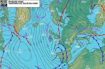
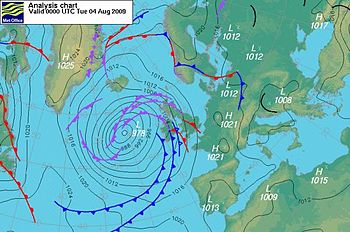
In atmospheric science, geostrophic flow is the theoretical wind that would result from an exact balance between the Coriolis force and the pressure gradient force. This condition is called geostrophic equilibrium or geostrophic balance. The geostrophic wind is directed parallel to isobars. This balance seldom holds exactly in nature. The true wind almost always differs from the geostrophic wind due to other forces such as friction from the ground. Thus, the actual wind would equal the geostrophic wind only if there were no friction and the isobars were perfectly straight. Despite this, much of the atmosphere outside the tropics is close to geostrophic flow much of the time and it is a valuable first approximation. Geostrophic flow in air or water is a zero-frequency inertial wave.

A Kelvin wave is a wave in the ocean or atmosphere that balances the Earth's Coriolis force against a topographic boundary such as a coastline, or a waveguide such as the equator. A feature of a Kelvin wave is that it is non-dispersive, i.e., the phase speed of the wave crests is equal to the group speed of the wave energy for all frequencies. This means that it retains its shape as it moves in the alongshore direction over time.

Thermal wind

The thermal wind is the vector difference between the geostrophic wind at upper altitudes minus that at lower altitudes in the atmosphere. It is the hypothetical vertical wind shear that would exist if the winds obey geostrophic balance in the horizontal, while pressure obeys hydrostatic balance in the vertical. The combination of these two force balances is called thermal wind balance, a term generalizable also to more complicated horizontal flow balances such as gradient wind balance.

The oceanic, wind driven Ekman spiral is the result of a force balance created by a shear stress force, Coriolis force and the water drag. This force balance gives a resulting current of the water different from the winds. In the ocean, there are two places where the Ekman spiral can be observed. At the surface of the ocean, where the shear stress force needed corresponds with the wind stress force and at the bottom of the ocean, where the shear stress force is created by friction with the ocean floor. This phenomenon was first observed at the surface by the Norwegian oceanographer Fridtjof Nansen during his Fram expedition. He noticed that icebergs did not drift in the same direction as the wind. His student, the Swedish oceanographer Vagn Walfrid Ekman, was the first person to physically explain this process.

Ekman transport Net transport of surface water perpendicular to wind direction

Ekman transport is part of Ekman motion theory, first investigated in 1902 by Vagn Walfrid Ekman. Winds are the main source of energy for ocean circulation, and Ekman Transport is a component of wind-driven ocean current. Ekman transport occurs when ocean surface waters are influenced by the friction force acting on them via the wind. As the wind blows it casts a friction force on the ocean surface that drags the upper 10-100m of the water column with it. However, due to the influence of the Coriolis effect, the ocean water moves at a 90° angle from the direction of the surface wind. The direction of transport is dependent on the hemisphere: in the northern hemisphere, transport occurs at 90° clockwise from wind direction, while in the southern hemisphere it occurs at 90° anticlockwise. This phenomenon was first noted by Fridtjof Nansen, who recorded that ice transport appeared to occur at an angle to the wind direction during his Arctic expedition during the 1890s. Ekman transport has significant impacts on the biogeochemical properties of the world's oceans. This is because it leads to upwelling and downwelling in order to obey mass conservation laws. Mass conservation, in reference to Ekman transfer, requires that any water displaced within an area must be replenished. This can be done by either Ekman suction or Ekman pumping depending on wind patterns.

In fluid mechanics, potential vorticity (PV) is a quantity which is proportional to the dot product of vorticity and stratification. This quantity, following a parcel of air or water, can only be changed by diabatic or frictional processes. It is a useful concept for understanding the generation of vorticity in cyclogenesis, especially along the polar front, and in analyzing flow in the ocean.

<span class="mw-page-title-main">Geostrophic current</span> Oceanic flow in which the pressure gradient force is balanced by the Coriolis effect

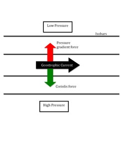
A geostrophic current is an oceanic current in which the pressure gradient force is balanced by the Coriolis effect. The direction of geostrophic flow is parallel to the isobars, with the high pressure to the right of the flow in the Northern Hemisphere, and the high pressure to the left in the Southern Hemisphere. This concept is familiar from weather maps, whose isobars show the direction of geostrophic winds. Geostrophic flow may be either barotropic or baroclinic. A geostrophic current may also be thought of as a rotating shallow water wave with a frequency of zero.

Inertial wave

Inertial waves, also known as inertial oscillations, are a type of mechanical wave possible in rotating fluids. Unlike surface gravity waves commonly seen at the beach or in the bathtub, inertial waves flow through the interior of the fluid, not at the surface. Like any other kind of wave, an inertial wave is caused by a restoring force and characterized by its wavelength and frequency. Because the restoring force for inertial waves is the Coriolis force, their wavelengths and frequencies are related in a peculiar way. Inertial waves are transverse. Most commonly they are observed in atmospheres, oceans, lakes, and laboratory experiments. Rossby waves, geostrophic currents, and geostrophic winds are examples of inertial waves. Inertial waves are also likely to exist in the molten core of the rotating Earth.

Frontogenesis is a meteorological process of tightening of horizontal temperature gradients to produce fronts. In the end, two types of fronts form: cold fronts and warm fronts. A cold front is a narrow line where temperature decreases rapidly. A warm front is a narrow line of warmer temperatures and essentially where much of the precipitation occurs. Frontogenesis occurs as a result of a developing baroclinic wave. According to Hoskins & Bretherton, there are eight mechanisms that influence temperature gradients: horizontal deformation, horizontal shearing, vertical deformation, differential vertical motion, latent heat release, surface friction, turbulence and mixing, and radiation. Semigeostrophic frontogenesis theory focuses on the role of horizontal deformation and shear.

In fluid dynamics, flow can be decomposed into primary plus secondary flow, a relatively weaker flow pattern superimposed on the stronger primary flow pattern. The primary flow is often chosen to be an exact solution to simplified or approximated governing equations, such as potential flow around a wing or geostrophic current or wind on the rotating Earth. In that case, the secondary flow usefully spotlights the effects of complicated real-world terms neglected in those approximated equations. For instance, the consequences of viscosity are spotlighted by secondary flow in the viscous boundary layer, resolving the tea leaf paradox. As another example, if the primary flow is taken to be a balanced flow approximation with net force equated to zero, then the secondary circulation helps spotlight acceleration due to the mild imbalance of forces. A smallness assumption about secondary flow also facilitates linearization.

The omega equation is a culminating result in synoptic-scale meteorology. It is an elliptic partial differential equation, named because its left-hand side produces an estimate of vertical velocity, customarily expressed by symbol , in a pressure coordinate measuring height the atmosphere. Mathematically, , where represents a material derivative. The underlying concept is more general, however, and can also be applied to the Boussinesq fluid equation system where vertical velocity is in altitude coordinate z.

Boundary current Ocean current with dynamics determined by the presence of a coastline

Boundary currents are ocean currents with dynamics determined by the presence of a coastline, and fall into two distinct categories: western boundary currents and eastern boundary currents.

Ocean dynamics define and describe the motion of water within the oceans. Ocean temperature and motion fields can be separated into three distinct layers: mixed (surface) layer, upper ocean, and deep ocean.

Equatorial Rossby waves, often called planetary waves, are very long, low frequency water waves found near the equator and are derived using the equatorial beta plane approximation.

Q-vectors are used in atmospheric dynamics to understand physical processes such as vertical motion and frontogenesis. Q-vectors are not physical quantities that can be measured in the atmosphere but are derived from the quasi-geostrophic equations and can be used in the previous diagnostic situations. On meteorological charts, Q-vectors point toward upward motion and away from downward motion. Q-vectors are an alternative to the omega equation for diagnosing vertical motion in the quasi-geostrophic equations.

While geostrophic motion refers to the wind that would result from an exact balance between the Coriolis force and horizontal pressure-gradient forces, quasi-geostrophic (QG) motion refers to flows where the Coriolis force and pressure gradient forces are almost in balance, but with inertia also having an effect.

A baroclinic instability is a fluid dynamical instability of fundamental importance in the atmosphere and ocean. It can lead to the formation of transient mesoscale eddies, with a horizontal scale of 10-100 km. In contrast, flows on the largest scale in the ocean are described as ocean currents, the largest scale eddies are mostly created by shearing of two ocean currents and static mesoscale eddies are formed by the flow around an obstacle (as seen in the animation on eddy. Mesoscale eddies are circular currents with swirling motion and account for approximately 90% of the ocean's total kinetic energy. Therefore, they are key in mixing and transport of for example heat, salt and nutrients.

Atmospheric circulation of a planet is largely specific to the planet in question and the study of atmospheric circulation of exoplanets is a nascent field as direct observations of exoplanet atmospheres are still quite sparse. However, by considering the fundamental principles of fluid dynamics and imposing various limiting assumptions, a theoretical understanding of atmospheric motions can be developed. This theoretical framework can also be applied to planets within the Solar System and compared against direct observations of these planets, which have been studied more extensively than exoplanets, to validate the theory and understand its limitations as well.

References

  1. Schaefer Etling, J.; C. Doswell (1980). "The Theory and Practical Application of Antitriptic Balance". Monthly Weather Review. 108 (6): 746–756. Bibcode:1980MWRv..108..746S. doi: 10.1175/1520-0493(1980)108<0746:TTAPAO>2.0.CO;2 . ISSN   1520-0493.
  2. Rennó, N.O.D.; H.B. Bluestein (2001). "A Simple Theory for Waterspouts". Journal of the Atmospheric Sciences. 58 (8): 927–932. Bibcode:2001JAtS...58..927R. doi:10.1175/1520-0469(2001)058<0927:ASTFW>2.0.CO;2. ISSN   1520-0469.
  3. Winn, W.P.; S.J. Hunyady G.D. Aulich (1999). "Pressure at the ground in a large tornado". Journal of Geophysical Research. 104 (D18): 22, 067–22, 082. Bibcode:1999JGR...10422067W. doi: 10.1029/1999JD900387 .

Further reading