CDF-based nonparametric confidence interval

Last updated July 24, 2023

In statistics, cumulative distribution function (CDF)-based nonparametric confidence intervals are a general class of confidence intervals around statistical functionals of a distribution. To calculate these confidence intervals, all that is required is an independently and identically distributed (iid) sample from the distribution and known bounds on the support of the distribution. The latter requirement simply means that all the nonzero probability mass of the distribution must be contained in some known interval $[a,b]$ .

Intuition

The intuition behind the CDF-based approach is that bounds on the CDF of a distribution can be translated into bounds on statistical functionals of that distribution. Given an upper and lower bound on the CDF, the approach involves finding the CDFs within the bounds that maximize and minimize the statistical functional of interest.

Properties of the bounds

Unlike approaches that make asymptotic assumptions, including bootstrap approaches and those that rely on the central limit theorem, CDF-based bounds are valid for finite sample sizes. And unlike bounds based on inequalities such as Hoeffding's and McDiarmid's inequalities, CDF-based bounds use properties of the entire sample and thus often produce significantly tighter bounds.

CDF bounds

When producing bounds on the CDF, we must differentiate between pointwise and simultaneous bands.

Pointwise band

A pointwise CDF bound is one which only guarantees their Coverage probability of $1-\alpha$ percent on any individual point of the empirical CDF. Because of the relaxed guarantees, these intervals can be much smaller.

One method of generating them is based on the Binomial distribution. Considering a single point of a CDF of value $F(x_{i})$ , then the empirical distribution at that point will be distributed proportional to the binomial distribution with $p=F(x_{i})$ and $n$ set equal to the number of samples in the empirical distribution. Thus, any of the methods available for generating a Binomial proportion confidence interval can be used to generate a CDF bound as well.

Simultaneous Band

CDF-based confidence intervals require a probabilistic bound on the CDF of the distribution from which the sample were generated. A variety of methods exist for generating confidence intervals for the CDF of a distribution, $F$ , given an i.i.d. sample drawn from the distribution. These methods are all based on the empirical distribution function (empirical CDF). Given an i.i.d. sample of size n, $x_{1},\ldots ,x_{n}\sim F$ , the empirical CDF is defined to be

{\hat {F}}_{n}(t)={\frac {1}{n}}\sum _{i=1}^{n}1\{x_{i}\leq t\},

where $1\{A\}$ is the indicator of event A. The Dvoretzky–Kiefer–Wolfowitz inequality,^[1] whose tight constant was determined by Massart,^[2] places a confidence interval around the Kolmogorov–Smirnov statistic between the CDF and the empirical CDF. Given an i.i.d. sample of size n from $F$ , the bound states

P(\sup _{x}|F(x)-F_{n}(x)|>\varepsilon )\leq 2e^{-2n\varepsilon ^{2}}.

This can be viewed as a confidence envelope that runs parallel to, and is equally above and below, the empirical CDF.

Illustration of the bound on the empirical CDF that is obtained using the Dvoretzky-Kiefer-Wolfowitz inequality. The notation
X
(
j
)
{\displaystyle X_{(j)}}
indicates the
j
th
{\displaystyle j^{\text{th}}}
order statistic. MassartBound.png — Illustration of the bound on the empirical CDF that is obtained using the Dvoretzky–Kiefer–Wolfowitz inequality. The notation $X_{(j)}$ indicates the $j^{\text{th}}$ order statistic.

The equally spaced confidence interval around the empirical CDF allows for different rates of violations across the support of the distribution. In particular, it is more common for a CDF to be outside of the CDF bound estimated using the Dvoretzky–Kiefer–Wolfowitz inequality near the median of the distribution than near the endpoints of the distribution. In contrast, the order statistics-based bound introduced by Learned-Miller and DeStefano^[3] allows for an equal rate of violation across all of the order statistics. This in turn results in a bound that is tighter near the ends of the support of the distribution and looser in the middle of the support. Other types of bounds can be generated by varying the rate of violation for the order statistics. For example, if a tighter bound on the distribution is desired on the upper portion of the support, a higher rate of violation can be allowed at the upper portion of the support at the expense of having a lower rate of violation, and thus a looser bound, for the lower portion of the support.

A nonparametric bound on the mean

Assume without loss of generality that the support of the distribution is contained in $[0,1].$ Given a confidence envelope for the CDF of $F$ it is easy to derive a corresponding confidence interval for the mean of $F$ . It can be shown^[4] that the CDF that maximizes the mean is the one that runs along the lower confidence envelope, $L(x)$ , and the CDF that minimizes the mean is the one that runs along the upper envelope, $U(x)$ . Using the identity

E(X)=\int _{0}^{1}(1-F(x))\,dx,

the confidence interval for the mean can be computed as

\left[\int _{0}^{1}(1-U(x))\,dx,\int _{0}^{1}(1-L(x))\,dx\right].

A nonparametric bound on the variance

Assume without loss of generality that the support of the distribution of interest, $F$ , is contained in $[0,1]$ . Given a confidence envelope for $F$ , it can be shown^[5] that the CDF within the envelope that minimizes the variance begins on the lower envelope, has a jump discontinuity to the upper envelope, and then continues along the upper envelope. Further, it can be shown that this variance-minimizing CDF, F', must satisfy the constraint that the jump discontinuity occurs at $E[F']$ . The variance maximizing CDF begins on the upper envelope, horizontally transitions to the lower envelope, then continues along the lower envelope. Explicit algorithms for calculating these variance-maximizing and minimizing CDFs are given by Romano and Wolf.^[5]

Bounds on other statistical functionals

The CDF-based framework for generating confidence intervals is very general and can be applied to a variety of other statistical functionals including

Entropy ^[3]
Mutual information ^[6]
Arbitrary percentiles

Related Research Articles

In probability theory and statistics, the binomial distribution with parameters n and p is the discrete probability distribution of the number of successes in a sequence of n independent experiments, each asking a yes–no question, and each with its own Boolean-valued outcome: success or failure. A single success/failure experiment is also called a Bernoulli trial or Bernoulli experiment, and a sequence of outcomes is called a Bernoulli process; for a single trial, i.e., n = 1, the binomial distribution is a Bernoulli distribution. The binomial distribution is the basis for the popular binomial test of statistical significance.

In statistics, the Kolmogorov–Smirnov test is a nonparametric test of the equality of continuous, one-dimensional probability distributions that can be used to compare a sample with a reference probability distribution, or to compare two samples. In essence, the test answers the question "How likely is it that we would see a collection of samples like this if they were drawn from that probability distribution?" or, in the second case, "How likely is it that we would see two sets of samples like this if they were drawn from the same probability distribution?". It is named after Andrey Kolmogorov and Nikolai Smirnov.

In statistics and probability theory, the median is the value separating the higher half from the lower half of a data sample, a population, or a probability distribution. For a data set, it may be thought of as "the middle" value. The basic feature of the median in describing data compared to the mean is that it is not skewed by a small proportion of extremely large or small values, and therefore provides a better representation of the center. Median income, for example, may be a better way to describe center of the income distribution because increases in the largest incomes alone have no effect on median. For this reason, the median is of central importance in robust statistics.

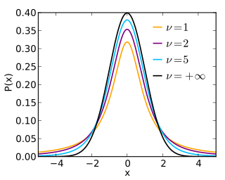
In probability and statistics, Student's t-distribution $is a continuous probability distribution that generalizes the standard normal distribution. Like the latter, it is symmetric around zero and bell-shaped.$

In probability theory, Chebyshev's inequality guarantees that, for a wide class of probability distributions, no more than a certain fraction of values can be more than a certain distance from the mean. Specifically, no more than 1/k² of the distribution's values can be k or more standard deviations away from the mean. The rule is often called Chebyshev's theorem, about the range of standard deviations around the mean, in statistics. The inequality has great utility because it can be applied to any probability distribution in which the mean and variance are defined. For example, it can be used to prove the weak law of large numbers.

In statistics, point estimation involves the use of sample data to calculate a single value which is to serve as a "best guess" or "best estimate" of an unknown population parameter. More formally, it is the application of a point estimator to the data to obtain a point estimate.

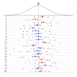
In frequentist statistics, a confidence interval (CI) is a range of estimates for an unknown parameter. A confidence interval is computed at a designated confidence level; the 95% confidence level is most common, but other levels, such as 90% or 99%, are sometimes used. The confidence level, degree of confidence or confidence coefficient represents the long-run proportion of CIs that theoretically contain the true value of the parameter; this is tantamount to the nominal coverage probability. For example, out of all intervals computed at the 95% level, 95% of them should contain the parameter's true value.

The standard error (SE) of a statistic is the standard deviation of its sampling distribution or an estimate of that standard deviation. If the statistic is the sample mean, it is called the standard error of the mean (SEM).

A tolerance interval (TI) is a statistical interval within which, with some confidence level, a specified sampled proportion of a population falls. "More specifically, a $100\times p %/100\times(1-α)$ tolerance interval provides limits within which at least a certain proportion (p) of the population falls with a given level of confidence (1−α)." "A (p, 1−α) tolerance interval (TI) based on a sample is constructed so that it would include at least a proportion p of the sampled population with confidence 1−α; such a TI is usually referred to as p-content − (1−α) coverage TI." "A (p, 1−α) upper tolerance limit (TL) is simply a 1−α upper confidence limit for the 100 p percentile of the population."

In probability theory, Hoeffding's inequality provides an upper bound on the probability that the sum of bounded independent random variables deviates from its expected value by more than a certain amount. Hoeffding's inequality was proven by Wassily Hoeffding in 1963.

In probability theory and statistics, the discrete uniform distribution is a symmetric probability distribution wherein a finite number of values are equally likely to be observed; every one of n values has equal probability 1/n. Another way of saying "discrete uniform distribution" would be "a known, finite number of outcomes equally likely to happen".

In probability theory and statistics, the continuous uniform distributions or rectangular distributions are a family of symmetric probability distributions. Such a distribution describes an experiment where there is an arbitrary outcome that lies between certain bounds. The bounds are defined by the parameters, $and which are the minimum and maximum values. The interval can either be closed or open. Therefore, the distribution is often abbreviated where stands for uniform distribution. The difference between the bounds defines the interval length; all intervals of the same length on the distribution's support are equally probable. It is the maximum entropy probability distribution for a random variable under no constraint other than that it is contained in the distribution's support.$

<span class="mw-page-title-main">Empirical distribution function</span> Distribution function associated with the empirical measure of a sample

In statistics, an empirical distribution function is the distribution function associated with the empirical measure of a sample. This cumulative distribution function is a step function that jumps up by $1/ n$ at each of the $n$ data points. Its value at any specified value of the measured variable is the fraction of observations of the measured variable that are less than or equal to the specified value.

In statistics, a binomial proportion confidence interval is a confidence interval for the probability of success calculated from the outcome of a series of success–failure experiments. In other words, a binomial proportion confidence interval is an interval estimate of a success probability p when only the number of experiments n and the number of successes n_S are known.

Bootstrapping is any test or metric that uses random sampling with replacement, and falls under the broader class of resampling methods. Bootstrapping assigns measures of accuracy to sample estimates. This technique allows estimation of the sampling distribution of almost any statistic using random sampling methods.

In the theory of probability and statistics, the Dvoretzky–Kiefer–Wolfowitz–Massart inequality bounds how close an empirically determined distribution function will be to the distribution function from which the empirical samples are drawn. It is named after Aryeh Dvoretzky, Jack Kiefer, and Jacob Wolfowitz, who in 1956 proved the inequality

A probability box is a characterization of uncertain numbers consisting of both aleatoric and epistemic uncertainties that is often used in risk analysis or quantitative uncertainty modeling where numerical calculations must be performed. Probability bounds analysis is used to make arithmetic and logical calculations with p-boxes.

In probability theory, the rectified Gaussian distribution is a modification of the Gaussian distribution when its negative elements are reset to 0. It is essentially a mixture of a discrete distribution and a continuous distribution as a result of censoring.

In probability theory, concentration inequalities provide bounds on how a random variable deviates from some value. The law of large numbers of classical probability theory states that sums of independent random variables are, under very mild conditions, close to their expectation with a large probability. Such sums are the most basic examples of random variables concentrated around their mean. Recent results show that such behavior is shared by other functions of independent random variables.

References

↑ A., Dvoretzky; Kiefer, J.; Wolfowitz, J. (1956). "Asymptotic minimax character of the sample distribution function and of the classical multinomial estimator". The Annals of Mathematical Statistics. 27 (3): 642–669. doi: 10.1214/aoms/1177728174 .
↑ Massart, P. (1990). "The tight constant in the Dvoretzky–Kiefer–Wolfowitz inequality". The Annals of Probability. 18 (3): 1269–1283. doi: 10.1214/aop/1176990746 .
1 2 Learned-Miller, E.; DeStefano, J. (2008). "A probabilistic upper bound on differential entropy". IEEE Transactions on Information Theory. 54 (11): 5223–5230. arXiv: cs/0504091 . doi:10.1109/tit.2008.929937. S2CID 1696031.
↑ Anderson, T.W. (1969). "Confidence limits for the value of an arbitrary bounded random variable with a continuous distribution function". Bulletin of the International and Statistical Institute. 43: 249–251.
1 2 Romano, J.P.; M., Wolf (2002). "Explicit nonparametric confidence intervals for the variance with guaranteed coverage". Communications in Statistics - Theory and Methods. 31 (8): 1231–1250. CiteSeerX 10.1.1.202.3170 . doi:10.1081/sta-120006065. S2CID 14330754.
↑ VanderKraats, N.D.; Banerjee, A. (2011). "A finite-sample, distribution-free, probabilistic lower bound on mutual information". Neural Computation. 23 (7): 1862–1898. doi:10.1162/neco_a_00144. PMID 21492010. S2CID 1736014.

This page is based on this Wikipedia article
Text is available under the CC BY-SA 4.0 license; additional terms may apply.
Images, videos and audio are available under their respective licenses.

[dvoretzky-1] A., Dvoretzky; Kiefer, J.; Wolfowitz, J. (1956). "Asymptotic minimax character of the sample distribution function and of the classical multinomial estimator". The Annals of Mathematical Statistics. 27 (3): 642–669. doi: 10.1214/aoms/1177728174 .

[massart-2] Massart, P. (1990). "The tight constant in the Dvoretzky–Kiefer–Wolfowitz inequality". The Annals of Probability. 18 (3): 1269–1283. doi: 10.1214/aop/1176990746 .

[entropy-3] 1 2 Learned-Miller, E.; DeStefano, J. (2008). "A probabilistic upper bound on differential entropy". IEEE Transactions on Information Theory. 54 (11): 5223–5230. arXiv: cs/0504091 . doi:10.1109/tit.2008.929937. S2CID 1696031.

[anderson-4] Anderson, T.W. (1969). "Confidence limits for the value of an arbitrary bounded random variable with a continuous distribution function". Bulletin of the International and Statistical Institute. 43: 249–251.

[romano2002explicit-5] 1 2 Romano, J.P.; M., Wolf (2002). "Explicit nonparametric confidence intervals for the variance with guaranteed coverage". Communications in Statistics - Theory and Methods. 31 (8): 1231–1250. CiteSeerX 10.1.1.202.3170 . doi:10.1081/sta-120006065. S2CID 14330754.

[mutualInformation-6] VanderKraats, N.D.; Banerjee, A. (2011). "A finite-sample, distribution-free, probabilistic lower bound on mutual information". Neural Computation. 23 (7): 1862–1898. doi:10.1162/neco_a_00144. PMID 21492010. S2CID 1736014.

[1]

[2]

[3]

[4]

[5]

[6]