This article assumes familiarity with the standard Lagrangian and Hamiltonian formalisms, and their connection to canonical quantization. Details of Dirac's modified Hamiltonian formalism are also summarized to put the Dirac bracket in context.
Inadequacy of the standard Hamiltonian procedure
The standard development of Hamiltonian mechanics is inadequate in several specific situations:
When the Lagrangian is at most linear in the velocity of at least one coordinate; in which case, the definition of the canonical momentum leads to a constraint. This is the most frequent reason to resort to Dirac brackets. For instance, the Lagrangian (density) for any fermion is of this form.
When there are gauge (or other unphysical) degrees of freedom which need to be fixed.
When there are any other constraints that one wishes to impose in phase space.
Example of a Lagrangian linear in velocity
An example in classical mechanics is a particle with charge q and mass m confined to the x - y plane with a strong constant, homogeneous perpendicular magnetic field, so then pointing in the z-direction with strength B.[4]
The Lagrangian for this system with an appropriate choice of parameters is
where →A is the vector potential for the magnetic field, →B; c is the speed of light in vacuum; and V(→r) is an arbitrary external scalar potential; one could easily take it to be quadratic in x and y, without loss of generality. We use
as our vector potential; this corresponds to a uniform and constant magnetic field B in the z direction. Here, the hats indicate unit vectors. Later in the article, however, they are used to distinguish quantum mechanical operators from their classical analogs. The usage should be clear from the context.
For a harmonic potential, the gradient of V amounts to just the coordinates, −(x,y).
Now, in the limit of a very large magnetic field, qB/mc ≫ 1. One may then drop the kinetic term to produce a simple approximate Lagrangian,
with first-order equations of motion
Note that this approximate Lagrangian is linear in the velocities, which is one of the conditions under which the standard Hamiltonian procedure breaks down. While this example has been motivated as an approximation, the Lagrangian under consideration is legitimate and leads to consistent equations of motion in the Lagrangian formalism.
Following the Hamiltonian procedure, however, the canonical momenta associated with the coordinates are now
which are unusual in that they are not invertible to the velocities; instead, they are constrained to be functions of the coordinates: the four phase-space variables are linearly dependent, so the variable basis is overcomplete.
Note that this "naive" Hamiltonian has no dependence on the momenta, which means that equations of motion (Hamilton's equations) are inconsistent.
The Hamiltonian procedure has broken down. One might try to fix the problem by eliminating two of the components of the 4-dimensional phase space, say y and py, down to a reduced phase space of 2 dimensions, that is sometimes expressing the coordinates as momenta and sometimes as coordinates. However, this is neither a general nor rigorous solution. This gets to the heart of the matter: that the definition of the canonical momenta implies a constraint on phase space (between momenta and coordinates) that was never taken into account.
Generalized Hamiltonian procedure
In Lagrangian mechanics, if the system has holonomic constraints, then one generally adds Lagrange multipliers to the Lagrangian to account for them. The extra terms vanish when the constraints are satisfied, thereby forcing the path of stationary action to be on the constraint surface. In this case, going to the Hamiltonian formalism introduces a constraint on phase space in Hamiltonian mechanics, but the solution is similar.
Before proceeding, it is useful to understand the notions of weak equality and strong equality. Two functions on phase space, f and g, are weakly equal if they are equal when the constraints are satisfied, but not throughout the phase space, denoted f ≈ g. If f and g are equal independently of the constraints being satisfied, they are called strongly equal, written f = g. It is important to note that, in order to get the right answer, no weak equations may be used before evaluating derivatives or Poisson brackets.
The new procedure works as follows, start with a Lagrangian and define the canonical momenta in the usual way. Some of those definitions may not be invertible and instead give a constraint in phase space (as above). Constraints derived in this way or imposed from the beginning of the problem are called primary constraints. The constraints, labeled φj, must weakly vanish, φj(p,q) ≈ 0.
Next, one finds the naive Hamiltonian, H, in the usual way via a Legendre transformation, exactly as in the above example. Note that the Hamiltonian can always be written as a function of qs and ps only, even if the velocities cannot be inverted into functions of the momenta.
Generalizing the Hamiltonian
Dirac argues that we should generalize the Hamiltonian (somewhat analogously to the method of Lagrange multipliers) to
where the cj are not constants but functions of the coordinates and momenta. Since this new Hamiltonian is the most general function of coordinates and momenta weakly equal to the naive Hamiltonian, H* is the broadest generalization of the Hamiltonian possible so that δH * ≈ δH when δφj ≈ 0.
To further illuminate the cj, consider how one gets the equations of motion from the naive Hamiltonian in the standard procedure. One expands the variation of the Hamiltonian out in two ways and sets them equal (using a somewhat abbreviated notation with suppressed indices and sums):
where the second equality holds after simplifying with the Euler-Lagrange equations of motion and the definition of canonical momentum. From this equality, one deduces the equations of motion in the Hamiltonian formalism from
where the weak equality symbol is no longer displayed explicitly, since by definition the equations of motion only hold weakly. In the present context, one cannot simply set the coefficients of δq and δp separately to zero, since the variations are somewhat restricted by the constraints. In particular, the variations must be tangent to the constraint surface.
One can demonstrate that the solution to
for the variations δqn and δpn restricted by the constraints Φj ≈ 0 (assuming the constraints satisfy some regularity conditions) is generally[5]
where the um are arbitrary functions.
Using this result, the equations of motion become
where the uk are functions of coordinates and velocities that can be determined, in principle, from the second equation of motion above.
The Legendre transform between the Lagrangian formalism and the Hamiltonian formalism has been saved at the cost of adding new variables.
Consistency conditions
The equations of motion become more compact when using the Poisson bracket, since if f is some function of the coordinates and momenta then
if one assumes that the Poisson bracket with the uk (functions of the velocity) exist; this causes no problems since the contribution weakly vanishes. Now, there are some consistency conditions which must be satisfied in order for this formalism to make sense. If the constraints are going to be satisfied, then their equations of motion must weakly vanish, that is, we require
There are four different types of conditions that can result from the above:
An equation that is inherently false, such as 1=0 .
An equation that is identically true, possibly after using one of our primary constraints.
An equation that places new constraints on our coordinates and momenta, but is independent of the uk.
An equation that serves to specify the uk.
The first case indicates that the starting Lagrangian gives inconsistent equations of motion, such as L = q. The second case does not contribute anything new.
The third case gives new constraints in phase space. A constraint derived in this manner is called a secondary constraint. Upon finding the secondary constraint one should add it to the extended Hamiltonian and check the new consistency conditions, which may result in still more constraints. Iterate this process until there are no more constraints. The distinction between primary and secondary constraints is largely an artificial one (i.e. a constraint for the same system can be primary or secondary depending on the Lagrangian), so this article does not distinguish between them from here on. Assuming the consistency condition has been iterated until all of the constraints have been found, then φj will index all of them. Note this article uses secondary constraint to mean any constraint that was not initially in the problem or derived from the definition of canonical momenta; some authors distinguish between secondary constraints, tertiary constraints, et cetera.
Finally, the last case helps fix the uk. If, at the end of this process, the uk are not completely determined, then that means there are unphysical (gauge) degrees of freedom in the system. Once all of the constraints (primary and secondary) are added to the naive Hamiltonian and the solutions to the consistency conditions for the uk are plugged in, the result is called the total Hamiltonian.
Determination of the uk
The uk must solve a set of inhomogeneous linear equations of the form
The above equation must possess at least one solution, since otherwise the initial Lagrangian is inconsistent; however, in systems with gauge degrees of freedom, the solution will not be unique. The most general solution is of the form
where Uk is a particular solution and Vk is the most general solution to the homogeneous equation
The most general solution will be a linear combination of linearly independent solutions to the above homogeneous equation. The number of linearly independent solutions equals the number of uk (which is the same as the number of constraints) minus the number of consistency conditions of the fourth type (in previous subsection). This is the number of unphysical degrees of freedom in the system. Labeling the linear independent solutions Vka where the index a runs from 1 to the number of unphysical degrees of freedom, the general solution to the consistency conditions is of the form
where the va are completely arbitrary functions of time. A different choice of the va corresponds to a gauge transformation, and should leave the physical state of the system unchanged.[6]
The total Hamiltonian
At this point, it is natural to introduce the total Hamiltonian
and what is denoted
The time evolution of a function on the phase space, f is governed by
Later, the extended Hamiltonian is introduced. For gauge-invariant (physically measurable quantities) quantities, all of the Hamiltonians should give the same time evolution, since they are all weakly equivalent. It is only for nongauge-invariant quantities that the distinction becomes important.
The Dirac bracket
Above is everything needed to find the equations of motion in Dirac's modified Hamiltonian procedure. Having the equations of motion, however, is not the endpoint for theoretical considerations. If one wants to canonically quantize a general system, then one needs the Dirac brackets. Before defining Dirac brackets, first-class and second-class constraints need to be introduced.
We call a function f(q, p) of coordinates and momenta first class if its Poisson bracket with all of the constraints weakly vanishes, that is,
for all j. Note that the only quantities that weakly vanish are the constraints φj, and therefore anything that weakly vanishes must be strongly equal to a linear combination of the constraints. One can demonstrate that the Poisson bracket of two first-class quantities must also be first class. The first-class constraints are intimately connected with the unphysical degrees of freedom mentioned earlier. Namely, the number of independent first-class constraints is equal to the number of unphysical degrees of freedom, and furthermore, the primary first-class constraints generate gauge transformations. Dirac further postulated that all secondary first-class constraints are generators of gauge transformations, which turns out to be false; however, typically one operates under the assumption that all first-class constraints generate gauge transformations when using this treatment.[7]
When the first-class secondary constraints are added into the Hamiltonian with arbitrary va as the first-class primary constraints are added to arrive at the total Hamiltonian, then one obtains the extended Hamiltonian. The extended Hamiltonian gives the most general possible time evolution for any gauge-dependent quantities, and may actually generalize the equations of motion from those of the Lagrangian formalism.
For the purposes of introducing the Dirac bracket, of more immediate interest are the second class constraints. Second class constraints are constraints that have a nonvanishing Poisson bracket with at least one other constraint.
For instance, consider second-class constraints φ1 and φ2 whose Poisson bracket is simply a constant, c,
Now, suppose one wishes to employ canonical quantization, then the phase-space coordinates become operators whose commutators become iħ times their classical Poisson bracket. Assuming there are no ordering issues that give rise to new quantum corrections, this implies that
where the hats emphasize the fact that the constraints are on operators.
On one hand, canonical quantization gives the above commutation relation, but on the other hand φ1 and φ2 are constraints that must vanish on physical states, whereas the right-hand side cannot vanish. This example illustrates the need for some generalization of the Poisson bracket which respects the system's constraints, and which leads to a consistent quantization procedure. This new bracket should be bilinear, antisymmetric, satisfy the Jacobi identity as does the Poisson bracket, reduce to the Poisson bracket for unconstrained systems, and, additionally, the bracket of any second-class constraint with any other quantity must vanish.
At this point, the second class constraints will be labeled . Define a matrix with entries
In this case, the Dirac bracket of two functions on phase space, f and g, is defined as
where M−1ab denotes the ab entry of M 's inverse matrix. Dirac proved that Mwill always be invertible.
It is straightforward to check that the above definition of the Dirac bracket satisfies all of the desired properties, and especially the last one, of vanishing for an argument which is a second-class constraint.
When applying canonical quantization on a constrained Hamiltonian system, the commutator of the operators is supplanted by iħ times their classical Dirac bracket. Since the Dirac bracket respects the constraints, one need not be careful about evaluating all brackets before using any weak equations, as is the case with the Poisson bracket.
Note that while the Poisson bracket of bosonic (Grassmann even) variables with itself must vanish, the Poisson bracket of fermions represented as a Grassmann variables with itself need not vanish. This means that in the fermionic case it is possible for there to be an odd number of second class constraints.
Illustration on the example provided
Returning to the above example, the naive Hamiltonian and the two primary constraints are
Therefore, the extended Hamiltonian can be written
The next step is to apply the consistency conditions {Φj, H*}PB ≈ 0, which in this case become
These are not secondary constraints, but conditions that fix u1 and u2. Therefore, there are no secondary constraints and the arbitrary coefficients are completely determined, indicating that there are no unphysical degrees of freedom.
If one plugs in with the values of u1 and u2, then one can see that the equations of motion are
which are self-consistent and coincide with the Lagrangian equations of motion.
A simple calculation confirms that φ1 and φ2 are second class constraints since
hence the matrix looks like
which is easily inverted to
where εab is the Levi-Civita symbol. Thus, the Dirac brackets are defined to be
If one always uses the Dirac bracket instead of the Poisson bracket, then there is no issue about the order of applying constraints and evaluating expressions, since the Dirac bracket of anything weakly zero is strongly equal to zero. This means that one can just use the naive Hamiltonian with Dirac brackets, instead, to thus get the correct equations of motion, which one can easily confirm on the above ones.
To quantize the system, the Dirac brackets between all of the phase space variables are needed. The nonvanishing Dirac brackets for this system are
while the cross-terms vanish, and
Therefore, the correct implementation of canonical quantization dictates the commutation relations,
with the cross terms vanishing, and
This example has a nonvanishing commutator between ∧x and ∧y, which means this structure specifies a noncommutative geometry. (Since the two coordinates do not commute, there will be an uncertainty principle for the x and y positions.)
Further Illustration for a hypersphere
Similarly, for free motion on a hypersphere Sn, the n + 1 coordinates are constrained, xi xi = 1. From a plain kinetic Lagrangian, it is evident that their momenta are perpendicular to them, xi pi = 0. Thus the corresponding Dirac Brackets are likewise simple to work out,[8]
The (2n + 1) constrained phase-space variables (xi, pi) obey much simpler Dirac brackets than the 2n unconstrained variables, had one eliminated one of the xs and one of the ps through the two constraints ab initio, which would obey plain Poisson brackets. The Dirac brackets add simplicity and elegance, at the cost of excessive (constrained) phase-space variables.
For example, for free motion on a circle, n = 1, for x1 ≡ z and eliminating x2 from the circle constraint yields the unconstrained
with equations of motion
an oscillation; whereas the equivalent constrained system with H = p2/2 = E yields
whence, instantly, virtually by inspection, oscillation for both variables,
The calculus of variations is a field of mathematical analysis that uses variations, which are small changes in functions and functionals, to find maxima and minima of functionals: mappings from a set of functions to the real numbers. Functionals are often expressed as definite integrals involving functions and their derivatives. Functions that maximize or minimize functionals may be found using the Euler–Lagrange equation of the calculus of variations.
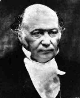
Hamiltonian mechanics emerged in 1833 as a reformulation of Lagrangian mechanics. Introduced by Sir William Rowan Hamilton, Hamiltonian mechanics replaces (generalized) velocities used in Lagrangian mechanics with (generalized) momenta. Both theories provide interpretations of classical mechanics and describe the same physical phenomena.
In mathematics and classical mechanics, the Poisson bracket is an important binary operation in Hamiltonian mechanics, playing a central role in Hamilton's equations of motion, which govern the time evolution of a Hamiltonian dynamical system. The Poisson bracket also distinguishes a certain class of coordinate transformations, called canonical transformations, which map canonical coordinate systems into canonical coordinate systems. A "canonical coordinate system" consists of canonical position and momentum variables that satisfy canonical Poisson bracket relations. The set of possible canonical transformations is always very rich. For instance, it is often possible to choose the Hamiltonian itself as one of the new canonical momentum coordinates.
In theoretical physics and mathematical physics, analytical mechanics, or theoretical mechanics is a collection of closely related alternative formulations of classical mechanics. It was developed by many scientists and mathematicians during the 18th century and onward, after Newtonian mechanics. Since Newtonian mechanics considers vector quantities of motion, particularly accelerations, momenta, forces, of the constituents of the system, an alternative name for the mechanics governed by Newton's laws and Euler's laws is vectorial mechanics.
In theoretical physics, the Batalin–Vilkovisky (BV) formalism was developed as a method for determining the ghost structure for Lagrangian gauge theories, such as gravity and supergravity, whose corresponding Hamiltonian formulation has constraints not related to a Lie algebra. The BV formalism, based on an action that contains both fields and "antifields", can be thought of as a vast generalization of the original BRST formalism for pure Yang–Mills theory to an arbitrary Lagrangian gauge theory. Other names for the Batalin–Vilkovisky formalism are field-antifield formalism, Lagrangian BRST formalism, or BV–BRST formalism. It should not be confused with the Batalin–Fradkin–Vilkovisky (BFV) formalism, which is the Hamiltonian counterpart.
In quantum mechanics, the canonical commutation relation is the fundamental relation between canonical conjugate quantities. For example,
In physics, canonical quantization is a procedure for quantizing a classical theory, while attempting to preserve the formal structure, such as symmetries, of the classical theory, to the greatest extent possible.
A first class constraint is a dynamical quantity in a constrained Hamiltonian system whose Poisson bracket with all the other constraints vanishes on the constraint surface in phase space. To calculate the first class constraint, one assumes that there are no second class constraints, or that they have been calculated previously, and their Dirac brackets generated.
In differential geometry, a field in mathematics, a Poisson manifold is a smooth manifold endowed with a Poisson structure. The notion of Poisson manifold generalises that of symplectic manifold, which in turn generalises the phase space from Hamiltonian mechanics.
In physics, the Hamilton–Jacobi equation, named after William Rowan Hamilton and Carl Gustav Jacob Jacobi, is an alternative formulation of classical mechanics, equivalent to other formulations such as Newton's laws of motion, Lagrangian mechanics and Hamiltonian mechanics.
In classical mechanics, Routh's procedure or Routhian mechanics is a hybrid formulation of Lagrangian mechanics and Hamiltonian mechanics developed by Edward John Routh. Correspondingly, the Routhian is the function which replaces both the Lagrangian and Hamiltonian functions. Routhian mechanics is equivalent to Lagrangian mechanics and Hamiltonian mechanics, and introduces no new physics. It offers an alternative way to solve mechanical problems.
In physics, canonical quantum gravity is an attempt to quantize the canonical formulation of general relativity. It is a Hamiltonian formulation of Einstein's general theory of relativity. The basic theory was outlined by Bryce DeWitt in a seminal 1967 paper, and based on earlier work by Peter G. Bergmann using the so-called canonical quantization techniques for constrained Hamiltonian systems invented by Paul Dirac. Dirac's approach allows the quantization of systems that include gauge symmetries using Hamiltonian techniques in a fixed gauge choice. Newer approaches based in part on the work of DeWitt and Dirac include the Hartle–Hawking state, Regge calculus, the Wheeler–DeWitt equation and loop quantum gravity.
In mechanics, a constant of motion is a quantity that is conserved throughout the motion, imposing in effect a constraint on the motion. However, it is a mathematical constraint, the natural consequence of the equations of motion, rather than a physical constraint. Common examples include energy, linear momentum, angular momentum and the Laplace–Runge–Lenz vector.
In physics, Lagrangian mechanics is a formulation of classical mechanics founded on the stationary-action principle. It was introduced by the Italian-French mathematician and astronomer Joseph-Louis Lagrange in his 1788 work, Mécanique analytique.
In analytical mechanics and quantum field theory, minimal coupling refers to a coupling between fields which involves only the charge distribution and not higher multipole moments of the charge distribution. This minimal coupling is in contrast to, for example, Pauli coupling, which includes the magnetic moment of an electron directly in the Lagrangian.
In quantum field theory, and in the significant subfields of quantum electrodynamics (QED) and quantum chromodynamics (QCD), the two-body Dirac equations (TBDE) of constraint dynamics provide a three-dimensional yet manifestly covariant reformulation of the Bethe–Salpeter equation for two spin-1/2 particles. Such a reformulation is necessary since without it, as shown by Nakanishi, the Bethe–Salpeter equation possesses negative-norm solutions arising from the presence of an essentially relativistic degree of freedom, the relative time. These "ghost" states have spoiled the naive interpretation of the Bethe–Salpeter equation as a quantum mechanical wave equation. The two-body Dirac equations of constraint dynamics rectify this flaw. The forms of these equations can not only be derived from quantum field theory they can also be derived purely in the context of Dirac's constraint dynamics and relativistic mechanics and quantum mechanics. Their structures, unlike the more familiar two-body Dirac equation of Breit, which is a single equation, are that of two simultaneous quantum relativistic wave equations. A single two-body Dirac equation similar to the Breit equation can be derived from the TBDE. Unlike the Breit equation, it is manifestly covariant and free from the types of singularities that prevent a strictly nonperturbative treatment of the Breit equation.
In physics and geometry, there are two closely related vector spaces, usually three-dimensional but in general of any finite dimension. Position space is the set of all position vectorsr in Euclidean space, and has dimensions of length; a position vector defines a point in space. Momentum space is the set of all momentum vectorsp a physical system can have; the momentum vector of a particle corresponds to its motion, with units of [mass][length][time]−1.
In the ADM formulation of general relativity one splits spacetime into spatial slices and time, the basic variables are taken to be the induced metric, , on the spatial slice, and its conjugate momentum variable related to the extrinsic curvature, ,. These are the metric canonical coordinates.
Lagrangian field theory is a formalism in classical field theory. It is the field-theoretic analogue of Lagrangian mechanics. Lagrangian mechanics is used to analyze the motion of a system of discrete particles each with a finite number of degrees of freedom. Lagrangian field theory applies to continua and fields, which have an infinite number of degrees of freedom.
In theoretical physics, Hamiltonian field theory is the field-theoretic analogue to classical Hamiltonian mechanics. It is a formalism in classical field theory alongside Lagrangian field theory. It also has applications in quantum field theory.
↑ See pages 48-58 of Ch. 2 in Henneaux, Marc and Teitelboim, Claudio, Quantization of Gauge Systems. Princeton University Press, 1992. ISBN0-691-08775-X
This page is based on this Wikipedia article Text is available under the CC BY-SA 4.0 license; additional terms may apply. Images, videos and audio are available under their respective licenses.