Gradient-enhanced kriging

Last updated

Gradient-enhanced kriging (GEK) is a surrogate modeling technique used in engineering. A surrogate model (alternatively known as a metamodel, response surface or emulator) is a prediction of the output of an expensive computer code. [1] This prediction is based on a small number of evaluations of the expensive computer code.

Contents

Introduction

Example of one-dimensional data interpolated by Kriging and GEK. The black line indicates the test-function, while the gray circles indicate 'observations', 'samples' or 'evaluations' of the test-function. The blue line is the Kriging mean, the shaded blue area illustrates the Kriging standard deviation. With GEK we can add the gradient information, illustrated in red, which increases the accuracy of the prediction. GEK test-function.png
Example of one-dimensional data interpolated by Kriging and GEK. The black line indicates the test-function, while the gray circles indicate 'observations', 'samples' or 'evaluations' of the test-function. The blue line is the Kriging mean, the shaded blue area illustrates the Kriging standard deviation. With GEK we can add the gradient information, illustrated in red, which increases the accuracy of the prediction.

Adjoint solvers are now becoming available in a range of computational fluid dynamics (CFD) solvers, such as Fluent, OpenFOAM, SU2 and US3D. Originally developed for optimization, adjoint solvers are now finding more and more use in uncertainty quantification.

Linear speedup

An adjoint solver allows one to compute the gradient of the quantity of interest with respect to all design parameters at the cost of one additional solve. This, potentially, leads to a linear speedup: the computational cost of constructing an accurate surrogate decrease, and the resulting computational speedup scales linearly with the number of design parameters.

The reasoning behind this linear speedup is straightforward. Assume we run primal solves and adjoint solves, at a total cost of . This results in data; values for the quantity of interest and partial derivatives in each of the gradients. Now assume that each partial derivative provides as much information for our surrogate as a single primal solve. Then, the total cost of getting the same amount of information from primal solves only is . The speedup is the ratio of these costs: [2] [3]

A linear speedup has been demonstrated for a fluid-structure interaction problem [2] and for a transonic airfoil. [3]

Noise

One issue with adjoint-based gradients in CFD is that they can be particularly noisy. [4] [5] When derived in a Bayesian framework, GEK allows one to incorporate not only the gradient information, but also the uncertainty in that gradient information. [6]

Approach

When using GEK one takes the following steps:

  1. Create a design of experiment (DoE): The DoE or 'sampling plan' is a list of different locations in the design space. The DoE indicates which combinations of parameters one will use to sample the computer simulation. With Kriging and GEK, a common choice is to use a Latin Hypercube Design (LHS) design with a 'maximin' criterion. The LHS-design is available in scripting codes like MATLAB or Python.
  2. Make observations: For each sample in our DoE one runs the computer simulation to obtain the Quantity of Interest (QoI).
  3. Construct the surrogate: One uses the GEK predictor equations to construct the surrogate conditional on the obtained observations.

Once the surrogate has been constructed it can be used in different ways, for example for surrogate-based uncertainty quantification (UQ) or optimization.

Predictor equations

In a Bayesian framework, we use Bayes' Theorem to predict the Kriging mean and covariance conditional on the observations. When using GEK, the observations are usually the results of a number of computer simulations. GEK can be interpreted as a form of Gaussian process regression.

Kriging

Along the lines of, [7] we are interested in the output of our computer simulation, for which we assume the normal prior probability distribution:

with prior mean and prior covariance matrix . The observations have the normal likelihood:

with the observation matrix and the observation error covariance matrix, which contains the observation uncertainties. After applying Bayes' Theorem we obtain a normally distributed posterior probability distribution, with Kriging mean:

and Kriging covariance:

where we have the gain matrix:

In Kriging, the prior covariance matrix is generated from a covariance function. One example of a covariance function is the Gaussian covariance:

where we sum over the dimensions and are the input parameters. The hyperparameters , and can be estimated from a Maximum Likelihood Estimate (MLE). [6] [8] [9]

Indirect GEK

There are several ways of implementing GEK. The first method, indirect GEK, defines a small but finite stepsize , and uses the gradient information to append synthetic data to the observations , see for example. [8] Indirect Kriging is sensitive to the choice of the step-size and cannot include observation uncertainties.

Direct GEK (through prior covariance matrix)

Direct GEK is a form of co-Kriging, where we add the gradient information as co-variables. This can be done by modifying the prior covariance or by modifying the observation matrix ; both approaches lead to the same GEK predictor. When we construct direct GEK through the prior covariance matrix, we append the partial derivatives to , and modify the prior covariance matrix such that it also contains the derivatives (and second derivatives) of the covariance function, see for example [10] . [6] The main advantages of direct GEK over indirect GEK are: 1) we do not have to choose a step-size, 2) we can include observation uncertainties for the gradients in , and 3) it is less susceptible to poor conditioning of the gain matrix . [6] [8]

Direct GEK (through observation matrix)

Another way of arriving at the same direct GEK predictor is to append the partial derivatives to the observations and include partial derivative operators in the observation matrix , see for example. [11]

Gradient-enhanced kriging for high-dimensional problems (Indirect method)

Current gradient-enhanced kriging methods do not scale well with the number of sampling points due to the rapid growth in the size of the correlation matrix, where new information is added for each sampling point in each direction of the design space. Furthermore, they do not scale well with the number of independent variables due to the increase in the number of hyperparameters that needs to be estimated. To address this issue, a new gradient-enhanced surrogate model approach that drastically reduced the number of hyperparameters through the use of the partial-least squares method that maintains accuracy is developed. In addition, this method is able to control the size of the correlation matrix by adding only relevant points defined through the information provided by the partial-least squares method. For more details, see. [12] This approach is implemented into the Surrogate Modeling Toolbox (SMT) in Python (https://github.com/SMTorg/SMT), and it runs on Linux, macOS, and Windows. SMT is distributed under the New BSD license.

Augmented gradient-enhanced kriging (direct method)

A universal augmented framework is proposed in [9] to append derivatives of any order to the observations. This method can be viewed as a generalization of Direct GEK that takes into account higher-order derivatives. Also, the observations and derivatives are not required to be measured at the same location under this framework.

Example: Drag coefficient of a transonic airfoil

Transonic airfoil. Transonic airfoil.png
Transonic airfoil.
Reference results for the drag coefficient of a transonic airfoil, based on a large number of CFD simulations. The horizontal and vertical axis show the deformation of the shape of the airfoil. GEK airfoil reference.png
Reference results for the drag coefficient of a transonic airfoil, based on a large number of CFD simulations. The horizontal and vertical axis show the deformation of the shape of the airfoil.
Kriging surrogate model of the drag coefficient of a transonic airfoil. The gray dots indicate the configurations for which the CFD solver was run. GEK airfoil Kriging.png
Kriging surrogate model of the drag coefficient of a transonic airfoil. The gray dots indicate the configurations for which the CFD solver was run.
GEK surrogate model of the drag coefficient of a transonic airfoil. The gray dots indicate the configurations for which the CFD solver was run, the arrows indicate the gradients. GEK airfoil GEK.png
GEK surrogate model of the drag coefficient of a transonic airfoil. The gray dots indicate the configurations for which the CFD solver was run, the arrows indicate the gradients.

As an example, consider the flow over a transonic airfoil. [3] The airfoil is operating at a Mach number of 0.8 and an angle of attack of 1.25 degrees. We assume that the shape of the airfoil is uncertain; the top and the bottom of the airfoil might have shifted up or down due to manufacturing tolerances. In other words, the shape of the airfoil that we are using might be slightly different from the airfoil that we designed.

On the right we see the reference results for the drag coefficient of the airfoil, based on a large number of CFD simulations. Note that the lowest drag, which corresponds to 'optimal' performance, is close to the undeformed 'baseline' design of the airfoil at (0,0).

After designing a sampling plan (indicated by the gray dots) and running the CFD solver at those sample locations, we obtain the Kriging surrogate model. The Kriging surrogate is close to the reference, but perhaps not as close as we would desire.

In the last figure, we have improved the accuracy of this surrogate model by including the adjoint-based gradient information, indicated by the arrows, and applying GEK.

Applications

GEK has found the following applications:

Related Research Articles

<span class="mw-page-title-main">Least squares</span> Approximation method in statistics

The method of least squares is a standard approach in regression analysis to approximate the solution of overdetermined systems by minimizing the sum of the squares of the residuals made in the results of each individual equation.

<span class="mw-page-title-main">Kalman filter</span> Algorithm that estimates unknowns from a series of measurements over time

For statistics and control theory, Kalman filtering, also known as linear quadratic estimation (LQE), is an algorithm that uses a series of measurements observed over time, including statistical noise and other inaccuracies, and produces estimates of unknown variables that tend to be more accurate than those based on a single measurement alone, by estimating a joint probability distribution over the variables for each timeframe. The filter is named after Rudolf E. Kálmán, who was one of the primary developers of its theory.

In probability theory and statistics, a Gaussian process is a stochastic process, such that every finite collection of those random variables has a multivariate normal distribution, i.e. every finite linear combination of them is normally distributed. The distribution of a Gaussian process is the joint distribution of all those random variables, and as such, it is a distribution over functions with a continuous domain, e.g. time or space.

<span class="mw-page-title-main">Computational fluid dynamics</span> Analysis and solving of problems that involve fluid flows

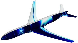
Computational fluid dynamics (CFD) is a branch of fluid mechanics that uses numerical analysis and data structures to analyze and solve problems that involve fluid flows. Computers are used to perform the calculations required to simulate the free-stream flow of the fluid, and the interaction of the fluid with surfaces defined by boundary conditions. With high-speed supercomputers, better solutions can be achieved, and are often required to solve the largest and most complex problems. Ongoing research yields software that improves the accuracy and speed of complex simulation scenarios such as transonic or turbulent flows. Initial validation of such software is typically performed using experimental apparatus such as wind tunnels. In addition, previously performed analytical or empirical analysis of a particular problem can be used for comparison. A final validation is often performed using full-scale testing, such as flight tests.

In mathematics, the Hessian matrix or Hessian is a square matrix of second-order partial derivatives of a scalar-valued function, or scalar field. It describes the local curvature of a function of many variables. The Hessian matrix was developed in the 19th century by the German mathematician Ludwig Otto Hesse and later named after him. Hesse originally used the term "functional determinants".

<span class="mw-page-title-main">Kriging</span> Method of interpolation

In statistics, originally in geostatistics, kriging or Kriging, also known as Gaussian process regression, is a method of interpolation based on Gaussian process governed by prior covariances. Under suitable assumptions of the prior, kriging gives the best linear unbiased prediction (BLUP) at unsampled locations. Interpolating methods based on other criteria such as smoothness may not yield the BLUP. The method is widely used in the domain of spatial analysis and computer experiments. The technique is also known as Wiener–Kolmogorov prediction, after Norbert Wiener and Andrey Kolmogorov.

In statistics, propagation of uncertainty is the effect of variables' uncertainties on the uncertainty of a function based on them. When the variables are the values of experimental measurements they have uncertainties due to measurement limitations which propagate due to the combination of variables in the function.

A computer experiment or simulation experiment is an experiment used to study a computer simulation, also referred to as an in silico system. This area includes computational physics, computational chemistry, computational biology and other similar disciplines.

Weighted least squares (WLS), also known as weighted linear regression, is a generalization of ordinary least squares and linear regression in which knowledge of the variance of observations is incorporated into the regression. WLS is also a specialization of generalized least squares.

<span class="mw-page-title-main">Turbulence modeling</span>

Turbulence modeling is the construction and use of a mathematical model to predict the effects of turbulence. Turbulent flows are commonplace in most real life scenarios, including the flow of blood through the cardiovascular system, the airflow over an aircraft wing, the re-entry of space vehicles, besides others. In spite of decades of research, there is no analytical theory to predict the evolution of these turbulent flows. The equations governing turbulent flows can only be solved directly for simple cases of flow. For most real life turbulent flows, CFD simulations use turbulent models to predict the evolution of turbulence. These turbulence models are simplified constitutive equations that predict the statistical evolution of turbulent flows.

Uncertainty quantification (UQ) is the science of quantitative characterization and reduction of uncertainties in both computational and real world applications. It tries to determine how likely certain outcomes are if some aspects of the system are not exactly known. An example would be to predict the acceleration of a human body in a head-on crash with another car: even if the speed was exactly known, small differences in the manufacturing of individual cars, how tightly every bolt has been tightened, etc., will lead to different results that can only be predicted in a statistical sense.

A surrogate model is an engineering method used when an outcome of interest cannot be easily measured or computed, so a model of the outcome is used instead. Most engineering design problems require experiments and/or simulations to evaluate design objective and constraint functions as a function of design variables. For example, in order to find the optimal airfoil shape for an aircraft wing, an engineer simulates the airflow around the wing for different shape variables. For many real-world problems, however, a single simulation can take many minutes, hours, or even days to complete. As a result, routine tasks such as design optimization, design space exploration, sensitivity analysis and what-if analysis become impossible since they require thousands or even millions of simulation evaluations.

Covariance matrix adaptation evolution strategy (CMA-ES) is a particular kind of strategy for numerical optimization. Evolution strategies (ES) are stochastic, derivative-free methods for numerical optimization of non-linear or non-convex continuous optimization problems. They belong to the class of evolutionary algorithms and evolutionary computation. An evolutionary algorithm is broadly based on the principle of biological evolution, namely the repeated interplay of variation and selection: in each generation (iteration) new individuals are generated by variation, usually in a stochastic way, of the current parental individuals. Then, some individuals are selected to become the parents in the next generation based on their fitness or objective function value . Like this, over the generation sequence, individuals with better and better -values are generated.

Polynomial chaos (PC), also called polynomial chaos expansion (PCE) and Wiener chaos expansion, is a method for representing a random variable in terms of a polynomial function of other random variables. The polynomials are chosen to be orthogonal with respect to the joint probability distribution of these random variables. PCE can be used, e.g., to determine the evolution of uncertainty in a dynamical system when there is probabilistic uncertainty in the system parameters. Note that despite its name, PCE has no immediate connections to chaos theory.

Natural evolution strategies (NES) are a family of numerical optimization algorithms for black box problems. Similar in spirit to evolution strategies, they iteratively update the (continuous) parameters of a search distribution by following the natural gradient towards higher expected fitness.

In applied statistics and geostatistics, regression-kriging (RK) is a spatial prediction technique that combines a regression of the dependent variable on auxiliary variables with interpolation (kriging) of the regression residuals. It is mathematically equivalent to the interpolation method variously called universal kriging and kriging with external drift, where auxiliary predictors are used directly to solve the kriging weights.

The quantum algorithm for linear systems of equations, also called HHL algorithm, designed by Aram Harrow, Avinatan Hassidim, and Seth Lloyd, is a quantum algorithm published in 2008 for solving linear systems. The algorithm estimates the result of a scalar measurement on the solution vector to a given linear system of equations.

This is a comparison of statistical analysis software that allows doing inference with Gaussian processes often using approximations.

Probabilistic numerics is a scientific field at the intersection of statistics, machine learning and applied mathematics, where tasks in numerical analysis including finding numerical solutions for integration, linear algebra, optimisation and differential equations are seen as problems of statistical, probabilistic, or Bayesian inference.

References

  1. Mitchell, M.; Morris, M. (1992). "Bayesian design and analysis of computer experiments: two examples" (PDF). Statistica Sinica (2): 359–379.
  2. 1 2 3 de Baar, J.H.S.; Scholcz, T.P.; Verhoosel, C.V.; Dwight, R.P.; van Zuijlen, A.H.; Bijl, H. (2012). "Efficient uncertainty quantification with gradient-enhanced Kriging: Applications in FSI" (PDF). ECCOMAS, Vienna, Austria, September 10–14.
  3. 1 2 3 4 de Baar, J.H.S.; Scholcz, T.P.; Dwight, R.P. (2015). "Exploiting Adjoint Derivatives in High-Dimensional Metamodels". AIAA Journal. 53 (5): 1391–1395. Bibcode:2015AIAAJ..53.1391D. doi:10.2514/1.J053678.
  4. Dwight, R.; Brezillon, J. (2006). "Effect of Approximations of the Discrete Adjoint on Gradient-Based Optimization". AIAA Journal. 44 (12): 3022–3031. Bibcode:2006AIAAJ..44.3022D. CiteSeerX   10.1.1.711.4761 . doi:10.2514/1.21744.
  5. Giles, M.; Duta, M.; Muller, J.; Pierce, N. (2003). "Algorithm Developments for Discrete Adjoint Methods". AIAA Journal. 41 (2): 198–205. Bibcode:2003AIAAJ..41..198G. doi:10.2514/2.1961. S2CID   2106397.
  6. 1 2 3 4 5 de Baar, J.H.S.; Dwight, R.P.; Bijl, H. (2014). "Improvements to gradient-enhanced Kriging using a Bayesian interpretation". International Journal for Uncertainty Quantification. 4 (3): 205–223. doi: 10.1615/Int.J.UncertaintyQuantification.2013006809 .
  7. Wikle, C.K.; Berliner, L.M. (2007). "A Bayesian tutorial for data assimilation". Physica D. 230 (1–2): 1–16. Bibcode:2007PhyD..230....1W. doi:10.1016/j.physd.2006.09.017.
  8. 1 2 3 4 Dwight, R.P.; Han, Z.-H. (2009). Efficient uncertainty quantification using gradient-enhanced Kriging (PDF). 11th AIAA Non-Deterministic Approaches Conference, Palm Springs, California, 4–7 May. doi:10.2514/6.2009-2276. ISBN   978-1-60086-975-4. S2CID   59019628.
  9. 1 2 Zhang, Sheng; Yang, Xiu; Tindel, Samy; Lin, Guang (2021). "Augmented Gaussian random field: Theory and computation". Discrete & Continuous Dynamical Systems - S. 15 (4): 931. arXiv: 2009.01961 . doi:10.3934/dcdss.2021098. S2CID   221507566.
  10. 1 2 Laurenceau, J.; Sagaut, P. (2008). "Building efficient response surfaces of aerodynamic functions with Kriging and coKriging". AIAA Journal. 46 (2): 498–507. Bibcode:2008AIAAJ..46..498L. doi:10.2514/1.32308. S2CID   17895486.
  11. de Baar, J.H.S. (2014). "Stochastic Surrogates for Measurements and Computer Models of Fluids". PhD Thesis, Delft University of Technology: 99–101.
  12. Bouhlel, M.A.; Martins, J.R.R.A. (2018). "Gradient-enhanced kriging for high-dimensional problems". Engineering with Computers. 35: 157–173. arXiv: 1708.02663 . doi:10.1007/s00366-018-0590-x. S2CID   3540630.
  13. Morris, M.D.; Mitchell, T.J.; Ylvisaker, D. (1993). "Bayesian Design and Analysis of Computer Experiments: Use of Derivatives in Surface Prediction". Technometrics. 35 (3): 243–255. doi:10.1080/00401706.1993.10485320.
  14. Chung, H.-S.; Alonso, J.J. (2002). "Using Gradients to Construct Cokriging Approximation Models for High-Dimensional Design Optimization Problems". AIAA 40th Aerospace Sciences Meeting and Exhibit: 2002–0317. CiteSeerX   10.1.1.12.4149 . doi:10.2514/6.2002-317.
  15. Han, Z.-H.; Gortz, S.; Zimmermann, R. (2013). "Improving variable-fidelity surrogate modeling via gradient-enhanced kriging and a generalized hybrid bridge function". Engineering with Computers. 32 (1): 15–34. doi:10.1016/j.ast.2012.01.006.
  16. Ulaganathan, S.; Couckuyt, I.; Dhaene, T.; Degroote, J.; Laermans, E. (2016). "Performance study of gradient-enhanced Kriging". Aerospace Science and Technology. 25 (1): 177–189.
  17. Laurent, L.; Le Riche, R.; Soulier, B.; Boucard, P.-A. (2017). "An overview of gradient-enhanced metamodels with applications" (PDF). Archives of Computational Methods in Engineering. 26: 1–46. doi:10.1007/s11831-017-9226-3. S2CID   54625655.
  18. Lockwood, B.A.; Anitescu, M. (2012). "Gradient-Enhanced Universal Kriging for Uncertainty Propagation" (PDF). Nuclear Science and Engineering. 170 (2): 168–195. CiteSeerX   10.1.1.187.6097 . doi:10.13182/NSE10-86. S2CID   18465024.
  19. Raggi, G.; Fdez. Galván, I.; Ritterhoff, C. L.; Vacher, M.; Lindh, R. (2020). "Restricted-Variance Molecular Geometry Optimization Based on Gradient-Enhanced Kriging". Journal of Chemical Theory and Computation. 16 (6): 3989–4001. doi: 10.1021/acs.jctc.0c00257 . PMC   7304864 . PMID   32374164.