Uncertainty quantification

Last updated

Uncertainty quantification (UQ) is the science of quantitative characterization and estimation of uncertainties in both computational and real world applications. It tries to determine how likely certain outcomes are if some aspects of the system are not exactly known. An example would be to predict the acceleration of a human body in a head-on crash with another car: even if the speed was exactly known, small differences in the manufacturing of individual cars, how tightly every bolt has been tightened, etc., will lead to different results that can only be predicted in a statistical sense.

Contents

Many problems in the natural sciences and engineering are also rife with sources of uncertainty. Computer experiments on computer simulations are the most common approach to study problems in uncertainty quantification. [1] [2] [3] [4]

Sources

Uncertainty can enter mathematical models and experimental measurements in various contexts. One way to categorize the sources of uncertainty is to consider: [5]

Parameter
This comes from the model parameters that are inputs to the computer model (mathematical model) but whose exact values are unknown to experimentalists and cannot be controlled in physical experiments, or whose values cannot be exactly inferred by statistical methods. Some examples of this are the local free-fall acceleration in a falling object experiment, various material properties in a finite element analysis for engineering, and multiplier uncertainty in the context of macroeconomic policy optimization.
Parametric
This comes from the variability of input variables of the model. For example, the dimensions of a work piece in a process of manufacture may not be exactly as designed and instructed, which would cause variability in its performance.
Structural uncertainty
Also known as model inadequacy, model bias, or model discrepancy, this comes from the lack of knowledge of the underlying physics in the problem. It depends on how accurately a mathematical model describes the true system for a real-life situation, considering the fact that models are almost always only approximations to reality. One example is when modeling the process of a falling object using the free-fall model; the model itself is inaccurate since there always exists air friction. In this case, even if there is no unknown parameter in the model, a discrepancy is still expected between the model and true physics.
Algorithmic
Also known as numerical uncertainty, or discrete uncertainty. This type comes from numerical errors and numerical approximations per implementation of the computer model. Most models are too complicated to solve exactly. For example, the finite element method or finite difference method may be used to approximate the solution of a partial differential equation (which introduces numerical errors). Other examples are numerical integration and infinite sum truncation that are necessary approximations in numerical implementation.
Experimental
Also known as observation error, this comes from the variability of experimental measurements. The experimental uncertainty is inevitable and can be noticed by repeating a measurement for many times using exactly the same settings for all inputs/variables.
Interpolation
This comes from a lack of available data collected from computer model simulations and/or experimental measurements. For other input settings that don't have simulation data or experimental measurements, one must interpolate or extrapolate in order to predict the corresponding responses.

Aleatoric and epistemic

Uncertainty is sometimes classified into two categories, [6] [7] prominently seen in medical applications. [8]

Aleatoric
Aleatoric uncertainty is also known as stochastic uncertainty, and is representative of unknowns that differ each time we run the same experiment. For example, a single arrow shot with a mechanical bow that exactly duplicates each launch (the same acceleration, altitude, direction and final velocity) will not all impact the same point on the target due to random and complicated vibrations of the arrow shaft, the knowledge of which cannot be determined sufficiently to eliminate the resulting scatter of impact points. The argument here is obviously in the definition of "cannot". Just because we cannot measure sufficiently with our currently available measurement devices does not preclude necessarily the existence of such information, which would move this uncertainty into the below category. Aleatoric is derived from the Latin alea or dice, referring to a game of chance.
Epistemic uncertainty
Epistemic uncertainty is also known as systematic uncertainty, and is due to things one could in principle know but does not in practice. This may be because a measurement is not accurate, because the model neglects certain effects, or because particular data have been deliberately hidden. An example of a source of this uncertainty would be the drag in an experiment designed to measure the acceleration of gravity near the earth's surface. The commonly used gravitational acceleration of 9.8 m/s² ignores the effects of air resistance, but the air resistance for the object could be measured and incorporated into the experiment to reduce the resulting uncertainty in the calculation of the gravitational acceleration.
Combined occurrence and interaction of aleatoric and epistemic uncertainty
Aleatoric and epistemic uncertainty can also occur simultaneously in a single term E.g., when experimental parameters show aleatoric uncertainty, and those experimental parameters are input to a computer simulation. If then for the uncertainty quantification a surrogate model, e.g. a Gaussian process or a Polynomial Chaos Expansion, is learnt from computer experiments, this surrogate exhibits epistemic uncertainty that depends on or interacts with the aleatoric uncertainty of the experimental parameters. [4] Such an uncertainty cannot solely be classified as aleatoric or epistemic any more, but is a more general inferential uncertainty.

In real life applications, both kinds of uncertainties are present. Uncertainty quantification intends to explicitly express both types of uncertainty separately. The quantification for the aleatoric uncertainties can be relatively straightforward, where traditional (frequentist) probability is the most basic form. Techniques such as the Monte Carlo method are frequently used. A probability distribution can be represented by its moments (in the Gaussian case, the mean and covariance suffice, although, in general, even knowledge of all moments to arbitrarily high order still does not specify the distribution function uniquely), or more recently, by techniques such as Karhunen–Loève and polynomial chaos expansions. To evaluate epistemic uncertainties, the efforts are made to understand the (lack of) knowledge of the system, process or mechanism. Epistemic uncertainty is generally understood through the lens of Bayesian probability, where probabilities are interpreted as indicating how certain a rational person could be regarding a specific claim.

Mathematical perspective

In mathematics, uncertainty is often characterized in terms of a probability distribution. From that perspective, epistemic uncertainty means not being certain what the relevant probability distribution is, and aleatoric uncertainty means not being certain what a random sample drawn from a probability distribution will be.

Types of problems

There are two major types of problems in uncertainty quantification: one is the forward propagation of uncertainty (where the various sources of uncertainty are propagated through the model to predict the overall uncertainty in the system response) and the other is the inverse assessment of model uncertainty and parameter uncertainty (where the model parameters are calibrated simultaneously using test data). There has been a proliferation of research on the former problem and a majority of uncertainty analysis techniques were developed for it. On the other hand, the latter problem is drawing increasing attention in the engineering design community, since uncertainty quantification of a model and the subsequent predictions of the true system response(s) are of great interest in designing robust systems.

Forward

Uncertainty propagation is the quantification of uncertainties in system output(s) propagated from uncertain inputs. It focuses on the influence on the outputs from the parametric variability listed in the sources of uncertainty. The targets of uncertainty propagation analysis can be:

Inverse

Given some experimental measurements of a system and some computer simulation results from its mathematical model, inverse uncertainty quantification estimates the discrepancy between the experiment and the mathematical model (which is called bias correction), and estimates the values of unknown parameters in the model if there are any (which is called parameter calibration or simply calibration). Generally this is a much more difficult problem than forward uncertainty propagation; however it is of great importance since it is typically implemented in a model updating process. There are several scenarios in inverse uncertainty quantification:

The outcome of bias correction, including an updated model (prediction mean) and prediction confidence interval. Bias Correction.png
The outcome of bias correction, including an updated model (prediction mean) and prediction confidence interval.

Bias correction only

Bias correction quantifies the model inadequacy, i.e. the discrepancy between the experiment and the mathematical model. The general model updating formula for bias correction is:

where denotes the experimental measurements as a function of several input variables , denotes the computer model (mathematical model) response, denotes the additive discrepancy function (aka bias function), and denotes the experimental uncertainty. The objective is to estimate the discrepancy function , and as a by-product, the resulting updated model is . A prediction confidence interval is provided with the updated model as the quantification of the uncertainty.

Parameter calibration only

Parameter calibration estimates the values of one or more unknown parameters in a mathematical model. The general model updating formulation for calibration is:

where denotes the computer model response that depends on several unknown model parameters , and denotes the true values of the unknown parameters in the course of experiments. The objective is to either estimate , or to come up with a probability distribution of that encompasses the best knowledge of the true parameter values.

Bias correction and parameter calibration

It considers an inaccurate model with one or more unknown parameters, and its model updating formulation combines the two together:

It is the most comprehensive model updating formulation that includes all possible sources of uncertainty, and it requires the most effort to solve.

Selective methodologies

Much research has been done to solve uncertainty quantification problems, though a majority of them deal with uncertainty propagation. During the past one to two decades, a number of approaches for inverse uncertainty quantification problems have also been developed and have proved to be useful for most small- to medium-scale problems.

Forward propagation

Existing uncertainty propagation approaches include probabilistic approaches and non-probabilistic approaches. There are basically six categories of probabilistic approaches for uncertainty propagation: [9]

For non-probabilistic approaches, interval analysis, [13] Fuzzy theory, Possibility theory and evidence theory are among the most widely used.

The probabilistic approach is considered as the most rigorous approach to uncertainty analysis in engineering design due to its consistency with the theory of decision analysis. Its cornerstone is the calculation of probability density functions for sampling statistics. [14] This can be performed rigorously for random variables that are obtainable as transformations of Gaussian variables, leading to exact confidence intervals.

Inverse uncertainty

Frequentist

In regression analysis and least squares problems, the standard error of parameter estimates is readily available, which can be expanded into a confidence interval.

Bayesian

Several methodologies for inverse uncertainty quantification exist under the Bayesian framework. The most complicated direction is to aim at solving problems with both bias correction and parameter calibration. The challenges of such problems include not only the influences from model inadequacy and parameter uncertainty, but also the lack of data from both computer simulations and experiments. A common situation is that the input settings are not the same over experiments and simulations. Another common situation is that parameters derived from experiments are input to simulations. For computationally expensive simulations, then often a surrogate model, e.g. a Gaussian process or a Polynomial Chaos Expansion, is necessary, defining an inverse problem for finding the surrogate model that best approximates the simulations. [4]

Modular approach

An approach to inverse uncertainty quantification is the modular Bayesian approach. [5] [15] The modular Bayesian approach derives its name from its four-module procedure. Apart from the current available data, a prior distribution of unknown parameters should be assigned.

Module 1: Gaussian process modeling for the computer model

To address the issue from lack of simulation results, the computer model is replaced with a Gaussian process (GP) model

where

is the dimension of input variables, and is the dimension of unknown parameters. While is pre-defined, , known as hyperparameters of the GP model, need to be estimated via maximum likelihood estimation (MLE). This module can be considered as a generalized kriging method.

Module 2: Gaussian process modeling for the discrepancy function

Similarly with the first module, the discrepancy function is replaced with a GP model

where

Together with the prior distribution of unknown parameters, and data from both computer models and experiments, one can derive the maximum likelihood estimates for . At the same time, from Module 1 gets updated as well.

Module 3: Posterior distribution of unknown parameters

Bayes' theorem is applied to calculate the posterior distribution of the unknown parameters:

where includes all the fixed hyperparameters in previous modules.

Module 4: Prediction of the experimental response and discrepancy function
Full approach

Fully Bayesian approach requires that not only the priors for unknown parameters but also the priors for the other hyperparameters should be assigned. It follows the following steps: [16]

  1. Derive the posterior distribution ;
  2. Integrate out and obtain . This single step accomplishes the calibration;
  3. Prediction of the experimental response and discrepancy function.

However, the approach has significant drawbacks:

  • For most cases, is a highly intractable function of . Hence the integration becomes very troublesome. Moreover, if priors for the other hyperparameters are not carefully chosen, the complexity in numerical integration increases even more.
  • In the prediction stage, the prediction (which should at least include the expected value of system responses) also requires numerical integration. Markov chain Monte Carlo (MCMC) is often used for integration; however it is computationally expensive.

The fully Bayesian approach requires a huge amount of calculations and may not yet be practical for dealing with the most complicated modelling situations. [16]

Known issues

The theories and methodologies for uncertainty propagation are much better established, compared with inverse uncertainty quantification. For the latter, several difficulties remain unsolved:

  1. Dimensionality issue: The computational cost increases dramatically with the dimensionality of the problem, i.e. the number of input variables and/or the number of unknown parameters.
  2. Identifiability issue: [17] Multiple combinations of unknown parameters and discrepancy function can yield the same experimental prediction. Hence different values of parameters cannot be distinguished/identified. This issue is circumvented in a Bayesian approach, where such combinations are averaged over. [4]
  3. Incomplete model response: Refers to a model not having a solution for some combinations of the input variables. [18] [19]
  4. Quantifying uncertainty in the input quantities: Crucial events missing in the available data or critical quantities unidentified to analysts due to, e.g., limitations in existing models. [20]
  5. Little consideration of the impact of choices made by analysts. [21]

See also

Related Research Articles

<span class="mw-page-title-main">Orbit</span> Curved path of an object around a point

In celestial mechanics, an orbit is the curved trajectory of an object such as the trajectory of a planet around a star, or of a natural satellite around a planet, or of an artificial satellite around an object or position in space such as a planet, moon, asteroid, or Lagrange point. Normally, orbit refers to a regularly repeating trajectory, although it may also refer to a non-repeating trajectory. To a close approximation, planets and satellites follow elliptic orbits, with the center of mass being orbited at a focal point of the ellipse, as described by Kepler's laws of planetary motion.

The likelihood function is the joint probability of observed data viewed as a function of the parameters of a statistical model.

<span class="mw-page-title-main">Navier–Stokes equations</span> Equations describing the motion of viscous fluid substances

The Navier–Stokes equations are partial differential equations which describe the motion of viscous fluid substances. They were named after French engineer and physicist Claude-Louis Navier and the Irish physicist and mathematician George Gabriel Stokes. They were developed over several decades of progressively building the theories, from 1822 (Navier) to 1842–1850 (Stokes).

Bayesian inference is a method of statistical inference in which Bayes' theorem is used to update the probability for a hypothesis as more evidence or information becomes available. Fundamentally, Bayesian inference uses prior knowledge, in the form of a prior distribution in order to estimate posterior probabilities. Bayesian inference is an important technique in statistics, and especially in mathematical statistics. Bayesian updating is particularly important in the dynamic analysis of a sequence of data. Bayesian inference has found application in a wide range of activities, including science, engineering, philosophy, medicine, sport, and law. In the philosophy of decision theory, Bayesian inference is closely related to subjective probability, often called "Bayesian probability".

Pattern recognition is the task of assigning a class to an observation based on patterns extracted from data. While similar, pattern recognition (PR) is not to be confused with pattern machines (PM) which may possess (PR) capabilities but their primary function is to distinguish and create emergent pattern. PR has applications in statistical data analysis, signal processing, image analysis, information retrieval, bioinformatics, data compression, computer graphics and machine learning. Pattern recognition has its origins in statistics and engineering; some modern approaches to pattern recognition include the use of machine learning, due to the increased availability of big data and a new abundance of processing power.

<span class="mw-page-title-main">Unit vector</span> Vector of length one

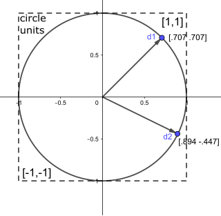
In mathematics, a unit vector in a normed vector space is a vector of length 1. A unit vector is often denoted by a lowercase letter with a circumflex, or "hat", as in .

<span class="mw-page-title-main">Logistic regression</span> Statistical model for a binary dependent variable

In statistics, the logistic model is a statistical model that models the log-odds of an event as a linear combination of one or more independent variables. In regression analysis, logistic regression is estimating the parameters of a logistic model. Formally, in binary logistic regression there is a single binary dependent variable, coded by an indicator variable, where the two values are labeled "0" and "1", while the independent variables can each be a binary variable or a continuous variable. The corresponding probability of the value labeled "1" can vary between 0 and 1, hence the labeling; the function that converts log-odds to probability is the logistic function, hence the name. The unit of measurement for the log-odds scale is called a logit, from logistic unit, hence the alternative names. See § Background and § Definition for formal mathematics, and § Example for a worked example.

<span class="mw-page-title-main">Loss function</span> Mathematical relation assigning a probability event to a cost

In mathematical optimization and decision theory, a loss function or cost function is a function that maps an event or values of one or more variables onto a real number intuitively representing some "cost" associated with the event. An optimization problem seeks to minimize a loss function. An objective function is either a loss function or its opposite, in which case it is to be maximized. The loss function could include terms from several levels of the hierarchy.

<span class="mw-page-title-main">Expectation–maximization algorithm</span> Iterative method for finding maximum likelihood estimates in statistical models

In statistics, an expectation–maximization (EM) algorithm is an iterative method to find (local) maximum likelihood or maximum a posteriori (MAP) estimates of parameters in statistical models, where the model depends on unobserved latent variables. The EM iteration alternates between performing an expectation (E) step, which creates a function for the expectation of the log-likelihood evaluated using the current estimate for the parameters, and a maximization (M) step, which computes parameters maximizing the expected log-likelihood found on the E step. These parameter-estimates are then used to determine the distribution of the latent variables in the next E step. It can be used, for example, to estimate a mixture of gaussians, or to solve the multiple linear regression problem.

In statistics, a generalized linear model (GLM) is a flexible generalization of ordinary linear regression. The GLM generalizes linear regression by allowing the linear model to be related to the response variable via a link function and by allowing the magnitude of the variance of each measurement to be a function of its predicted value.

In statistics, the theory of minimum norm quadratic unbiased estimation (MINQUE) was developed by C. R. Rao. MINQUE is a theory alongside other estimation methods in estimation theory, such as the method of moments or maximum likelihood estimation. Similar to the theory of best linear unbiased estimation, MINQUE is specifically concerned with linear regression models. The method was originally conceived to estimate heteroscedastic error variance in multiple linear regression. MINQUE estimators also provide an alternative to maximum likelihood estimators or restricted maximum likelihood estimators for variance components in mixed effects models. MINQUE estimators are quadratic forms of the response variable and are used to estimate a linear function of the variances.

<span class="mw-page-title-main">Ornstein–Uhlenbeck process</span> Stochastic process modeling random walk with friction

In mathematics, the Ornstein–Uhlenbeck process is a stochastic process with applications in financial mathematics and the physical sciences. Its original application in physics was as a model for the velocity of a massive Brownian particle under the influence of friction. It is named after Leonard Ornstein and George Eugene Uhlenbeck.

In statistics, the generalized linear array model (GLAM) is used for analyzing data sets with array structures. It based on the generalized linear model with the design matrix written as a Kronecker product.

Non-linear least squares is the form of least squares analysis used to fit a set of m observations with a model that is non-linear in n unknown parameters (m ≥ n). It is used in some forms of nonlinear regression. The basis of the method is to approximate the model by a linear one and to refine the parameters by successive iterations. There are many similarities to linear least squares, but also some significant differences. In economic theory, the non-linear least squares method is applied in (i) the probit regression, (ii) threshold regression, (iii) smooth regression, (iv) logistic link regression, (v) Box–Cox transformed regressors ().

Gradient-enhanced kriging (GEK) is a surrogate modeling technique used in engineering. A surrogate model is a prediction of the output of an expensive computer code. This prediction is based on a small number of evaluations of the expensive computer code.

SAMV is a parameter-free superresolution algorithm for the linear inverse problem in spectral estimation, direction-of-arrival (DOA) estimation and tomographic reconstruction with applications in signal processing, medical imaging and remote sensing. The name was coined in 2013 to emphasize its basis on the asymptotically minimum variance (AMV) criterion. It is a powerful tool for the recovery of both the amplitude and frequency characteristics of multiple highly correlated sources in challenging environments. Applications include synthetic-aperture radar, computed tomography scan, and magnetic resonance imaging (MRI).

<span class="mw-page-title-main">Stochastic gradient Langevin dynamics</span>

Stochastic gradient Langevin dynamics (SGLD) is an optimization and sampling technique composed of characteristics from Stochastic gradient descent, a Robbins–Monro optimization algorithm, and Langevin dynamics, a mathematical extension of molecular dynamics models. Like stochastic gradient descent, SGLD is an iterative optimization algorithm which uses minibatching to create a stochastic gradient estimator, as used in SGD to optimize a differentiable objective function. Unlike traditional SGD, SGLD can be used for Bayesian learning as a sampling method. SGLD may be viewed as Langevin dynamics applied to posterior distributions, but the key difference is that the likelihood gradient terms are minibatched, like in SGD. SGLD, like Langevin dynamics, produces samples from a posterior distribution of parameters based on available data. First described by Welling and Teh in 2011, the method has applications in many contexts which require optimization, and is most notably applied in machine learning problems.

<span class="mw-page-title-main">Hyperbolastic functions</span> Mathematical functions

The hyperbolastic functions, also known as hyperbolastic growth models, are mathematical functions that are used in medical statistical modeling. These models were originally developed to capture the growth dynamics of multicellular tumor spheres, and were introduced in 2005 by Mohammad Tabatabai, David Williams, and Zoran Bursac. The precision of hyperbolastic functions in modeling real world problems is somewhat due to their flexibility in their point of inflection. These functions can be used in a wide variety of modeling problems such as tumor growth, stem cell proliferation, pharma kinetics, cancer growth, sigmoid activation function in neural networks, and epidemiological disease progression or regression.

Bayesian history matching is a statistical method for calibrating complex computer models. The equations inside many scientific computer models contain parameters which have a true value, but that true value is often unknown; history matching is one technique for learning what these parameters could be.

Integrated nested Laplace approximations (INLA) is a method for approximate Bayesian inference based on Laplace's method. It is designed for a class of models called latent Gaussian models (LGMs), for which it can be a fast and accurate alternative for Markov chain Monte Carlo methods to compute posterior marginal distributions. Due to its relative speed even with large data sets for certain problems and models, INLA has been a popular inference method in applied statistics, in particular spatial statistics, ecology, and epidemiology. It is also possible to combine INLA with a finite element method solution of a stochastic partial differential equation to study e.g. spatial point processes and species distribution models. The INLA method is implemented in the R-INLA R package.

References

  1. Sacks, Jerome; Welch, William J.; Mitchell, Toby J.; Wynn, Henry P. (1989). "Design and Analysis of Computer Experiments". Statistical Science. 4 (4): 409–423. doi: 10.1214/ss/1177012413 . JSTOR   2245858.
  2. Iman, Ronald L.; Helton, Jon C. (1988). "An Investigation of Uncertainty and Sensitivity Analysis Techniques for Computer Models". Risk Analysis. Wiley. 8 (1): 71–90. Bibcode:1988RiskA...8...71I. doi:10.1111/j.1539-6924.1988.tb01155.x. ISSN   0272-4332.
  3. Walker, W.E.; Harremoës, P.; Rotmans, J.; van der Sluijs, J.P.; van Asselt, M.B.A.; Janssen, P.; Krayer von Krauss, M.P. (2003). "Defining Uncertainty: A Conceptual Basis for Uncertainty Management in Model-Based Decision Support". Integrated Assessment. Swets & Zeitlinger Publishers. 4 (1): 5–17. Bibcode:2003IntAs...4....5W. doi:10.1076/iaij.4.1.5.16466. hdl: 1874/386032 . ISSN   1389-5176.
  4. 1 2 3 4 5 Ranftl, Sascha; von der Linden, Wolfgang (2021-11-13). "Bayesian Surrogate Analysis and Uncertainty Propagation". Physical Sciences Forum. 3 (1): 6. arXiv: 2101.04038 . doi: 10.3390/psf2021003006 . ISSN   2673-9984.
  5. 1 2 Kennedy, Marc C.; O'Hagan, Anthony (2001). "Bayesian calibration of computer models". Journal of the Royal Statistical Society, Series B (Statistical Methodology). 63 (3): 425–464. doi: 10.1111/1467-9868.00294 .
  6. Der Kiureghian, Armen; Ditlevsen, Ove (2009). "Aleatory or epistemic? Does it matter?". Structural Safety. 31 (2): 105–112. doi:10.1016/j.strusafe.2008.06.020.
  7. Matthies, Hermann G. (2007). "Quantifying Uncertainty: Modern Computational Representation of Probability and Applications". Extreme Man-Made and Natural Hazards in Dynamics of Structures. NATO Security through Science Series. pp. 105–135. doi:10.1007/978-1-4020-5656-7_4. ISBN   978-1-4020-5654-3.
  8. Abhaya Indrayan, Medical Biostatistics, Second Edition, Chapman & Hall/CRC Press, 2008, pages 8, 673
  9. Lee, S. H.; Chen, W. (2008-05-09). "A comparative study of uncertainty propagation methods for black-box-type problems". Structural and Multidisciplinary Optimization. Springer Science and Business Media LLC. 37 (3): 239–253. doi:10.1007/s00158-008-0234-7. ISSN   1615-147X. S2CID   119988015.
  10. Cardenas, IC (2019). "On the use of Bayesian networks as a meta-modeling approach to analyse uncertainties in slope stability analysis". Georisk: Assessment and Management of Risk for Engineered Systems and Geohazards. 13 (1): 53–65. Bibcode:2019GAMRE..13...53C. doi:10.1080/17499518.2018.1498524. S2CID   216590427.
  11. Ranftl, Sascha; Melito, Gian Marco; Badeli, Vahid; Reinbacher-Köstinger, Alice; Ellermann, Katrin; von der Linden, Wolfgang (2019-12-31). "Bayesian Uncertainty Quantification with Multi-Fidelity Data and Gaussian Processes for Impedance Cardiography of Aortic Dissection". Entropy. 22 (1): 58. Bibcode:2019Entrp..22...58R. doi: 10.3390/e22010058 . ISSN   1099-4300. PMC   7516489 . PMID   33285833.
  12. Ranftl, Sascha; Müller, Thomas Stephan; Windberger, Ursula; von der Linden, Wolfgang; Brenn, Günter (2021-05-03), Data and codes for 'A Bayesian Approach to Blood Rheological Uncertainties in Aortic Hemodynamics', doi:10.5281/zenodo.5237189 , retrieved 2022-01-12
  13. Jaulin, L.; Kieffer, M.; Didrit, O.; Walter, E. (2001). Applied Interval Analysis. Springer. ISBN   1-85233-219-0.
  14. Arnaut, L. R. Measurement uncertainty in reverberation chambers - I. Sample statistics. Technical report TQE 2, 2nd. ed., sec. 3.1, National Physical Laboratory, 2008.
  15. Marc C. Kennedy, Anthony O'Hagan, Supplementary Details on Bayesian Calibration of Computer Models, Sheffield, University of Sheffield: 1–13, 2000
  16. 1 2 Bayarri, M. J.; Berger, J. O.; Liu, F. (2009-03-01). "Modularization in Bayesian analysis, with emphasis on analysis of computer models". Bayesian Analysis. Institute of Mathematical Statistics. 4 (1): 119–150. doi: 10.1214/09-ba404 . ISSN   1936-0975.
  17. Arendt, Paul D.; Apley, Daniel W.; Chen, Wei; Lamb, David; Gorsich, David (2012-09-28). "Improving Identifiability in Model Calibration Using Multiple Responses". Journal of Mechanical Design. ASME International. 134 (10): 100909. doi:10.1115/1.4007573. ISSN   1050-0472.
  18. Cardenas, IC (2019). "On the use of Bayesian networks as a meta-modeling approach to analyse uncertainties in slope stability analysis". Georisk: Assessment and Management of Risk for Engineered Systems and Geohazards. 13 (1): 53–65. Bibcode:2019GAMRE..13...53C. doi:10.1080/17499518.2018.1498524. S2CID   216590427.
  19. van den Eijnden, AP; Schweckendiek, T; Hicks, MA (2021). "Metamodelling for geotechnical reliability analysis with noisy and incomplete models". Georisk: Assessment and Management of Risk for Engineered Systems and Geohazards. 16 (3): 518–535. doi: 10.1080/17499518.2021.1952611 . S2CID   238819106.
  20. Cardenas, I.; Aven, T.; Flage, R. (2022). "Addressing challenges in uncertainty quantification. The case of geohazard assessments". Geosci. Model Dev. Discuss. 16 (6): 1601–1615. doi: 10.5194/gmd-16-1601-2023 . hdl: 11250/3105739 .
  21. Cardenas, I.; Aven, T.; Flage, R. (2022). "Addressing challenges in uncertainty quantification. The case of geohazard assessments". Geosci. Model Dev. Discuss. 16 (6): 1601–1615. doi: 10.5194/gmd-16-1601-2023 . hdl: 11250/3105739 .