If F is the only force acting on the system, the system is called a simple harmonic oscillator, and it undergoes simple harmonic motion: sinusoidaloscillations about the equilibrium point, with a constant amplitude and a constant frequency (which does not depend on the amplitude).
If a frictional force (damping) proportional to the velocity is also present, the harmonic oscillator is described as a damped oscillator. Depending on the friction coefficient, the system can:
Oscillate with a frequency lower than in the undamped case, and an amplitude decreasing with time (underdamped oscillator).
Decay to the equilibrium position, without oscillations (overdamped oscillator).
The boundary solution between an underdamped oscillator and an overdamped oscillator occurs at a particular value of the friction coefficient and is called critically damped.
If an external time-dependent force is present, the harmonic oscillator is described as a driven oscillator.
Mechanical examples include pendulums (with small angles of displacement), masses connected to springs, and acoustical systems. Other analogous systems include electrical harmonic oscillators such as RLC circuits. The harmonic oscillator model is very important in physics, because any mass subject to a force in stable equilibrium acts as a harmonic oscillator for small vibrations. Harmonic oscillators occur widely in nature and are exploited in many manmade devices, such as clocks and radio circuits. They are the source of virtually all sinusoidal vibrations and waves.
A simple harmonic oscillator is an oscillator that is neither driven nor damped. It consists of a mass m, which experiences a single force F, which pulls the mass in the direction of the point x = 0 and depends only on the position x of the mass and a constant k. Balance of forces (Newton's second law) for the system is
Solving this differential equation, we find that the motion is described by the function
where
The motion is periodic, repeating itself in a sinusoidal fashion with constant amplitude A. In addition to its amplitude, the motion of a simple harmonic oscillator is characterized by its period, the time for a single oscillation or its frequency , the number of cycles per unit time. The position at a given time t also depends on the phaseφ, which determines the starting point on the sine wave. The period and frequency are determined by the size of the mass m and the force constant k, while the amplitude and phase are determined by the starting position and velocity.
The velocity and acceleration of a simple harmonic oscillator oscillate with the same frequency as the position, but with shifted phases. The velocity is maximal for zero displacement, while the acceleration is in the direction opposite to the displacement.
The potential energy stored in a simple harmonic oscillator at position x is
Dependence of the system behavior on the value of the damping ratio ζPhase portrait of damped oscillator, with increasing damping strength.Video clip demonstrating a damped harmonic oscillator consisting of a dynamics cart between two springs. An accelerometer on top of the cart shows the magnitude and direction of the acceleration.
In real oscillators, friction, or damping, slows the motion of the system. Due to frictional force, the velocity decreases in proportion to the acting frictional force. While in a simple undriven harmonic oscillator the only force acting on the mass is the restoring force, in a damped harmonic oscillator there is in addition a frictional force which is always in a direction to oppose the motion. In many vibrating systems the frictional force Ff can be modeled as being proportional to the velocity v of the object: Ff = −cv, where c is called the viscous damping coefficient.
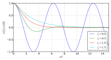
Step response of a damped harmonic oscillator; curves are plotted for three values of μ = ω1 = ω0√1 − ζ. Time is in units of the decay time τ = 1/(ζω0).
The value of the damping ratio ζ critically determines the behavior of the system. A damped harmonic oscillator can be:
Overdamped (ζ > 1): The system returns (exponentially decays) to steady state without oscillating. Larger values of the damping ratio ζ return to equilibrium more slowly.
Critically damped (ζ = 1): The system returns to steady state as quickly as possible without oscillating (although overshoot can occur if the initial velocity is nonzero). This is often desired for the damping of systems such as doors.
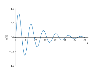
Underdamped (ζ < 1): The system oscillates (with a slightly different frequency than the undamped case) with the amplitude gradually decreasing to zero. The angular frequency of the underdamped harmonic oscillator is given by the exponential decay of the underdamped harmonic oscillator is given by
In the case ζ < 1 and a unit step input withx(0) = 0:
the solution is
with phase φ given by
The time an oscillator needs to adapt to changed external conditions is of the order τ = 1/(ζω0). In physics, the adaptation is called relaxation, and τ is called the relaxation time.
In electrical engineering, a multiple of τ is called the settling time, i.e. the time necessary to ensure the signal is within a fixed departure from final value, typically within 10%. The term overshoot refers to the extent the response maximum exceeds final value, and undershoot refers to the extent the response falls below final value for times following the response maximum.
Sinusoidal driving force
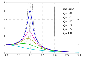
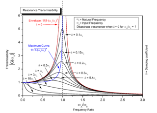
Steady-state variation of amplitude with relative frequency and damping of a driven harmonic oscillator. This plot is also called the harmonic oscillator spectrum or motional spectrum.
In the case of a sinusoidal driving force:
where is the driving amplitude, and is the driving frequency for a sinusoidal driving mechanism. This type of system appears in AC-driven RLC circuits (resistor–inductor–capacitor) and driven spring systems having internal mechanical resistance or external air resistance.
The general solution is a sum of a transient solution that depends on initial conditions, and a steady state that is independent of initial conditions and depends only on the driving amplitude , driving frequency , undamped angular frequency , and the damping ratio .
The steady-state solution is proportional to the driving force with an induced phase change :
is the phase of the oscillation relative to the driving force. The phase value is usually taken to be between −180° and 0 (that is, it represents a phase lag, for both positive and negative values of the arctan argument).
For a particular driving frequency called the resonance, or resonant frequency , the amplitude (for a given ) is maximal. This resonance effect only occurs when , i.e. for significantly underdamped systems. For strongly underdamped systems the value of the amplitude can become quite large near the resonant frequency.
The transient solutions are the same as the unforced () damped harmonic oscillator and represent the systems response to other events that occurred previously. The transient solutions typically die out rapidly enough that they can be ignored.
A parametric oscillator is a driven harmonic oscillator in which the drive energy is provided by varying the parameters of the oscillator, such as the damping or restoring force. A familiar example of parametric oscillation is "pumping" on a playground swing.[4][5][6] A person on a moving swing can increase the amplitude of the swing's oscillations without any external drive force (pushes) being applied, by changing the moment of inertia of the swing by rocking back and forth ("pumping") or alternately standing and squatting, in rhythm with the swing's oscillations. The varying of the parameters drives the system. Examples of parameters that may be varied are its resonance frequency and damping .
Parametric oscillators are used in many applications. The classical varactor parametric oscillator oscillates when the diode's capacitance is varied periodically. The circuit that varies the diode's capacitance is called the "pump" or "driver". In microwave electronics, waveguide/YAG based parametric oscillators operate in the same fashion. The designer varies a parameter periodically to induce oscillations.
Parametric oscillators have been developed as low-noise amplifiers, especially in the radio and microwave frequency range. Thermal noise is minimal, since a reactance (not a resistance) is varied. Another common use is frequency conversion, e.g., conversion from audio to radio frequencies. For example, the Optical parametric oscillator converts an input laser wave into two output waves of lower frequency ().
Parametric resonance occurs in a mechanical system when a system is parametrically excited and oscillates at one of its resonant frequencies. Parametric excitation differs from forcing, since the action appears as a time varying modification on a system parameter. This effect is different from regular resonance because it exhibits the instability phenomenon.
Universal oscillator equation
The equation
is known as the universal oscillator equation, since all second-order linear oscillatory systems can be reduced to this form.[citation needed] This is done through nondimensionalization.
If the forcing function is f(t) = cos(ωt) = cos(ωtcτ) = cos(ωτ), where ω = ωtc, the equation becomes
The solution to this differential equation contains two parts: the "transient" and the "steady-state".
The transient solution is independent of the forcing function.
Steady-state solution
Apply the "complex variables method" by solving the auxiliary equation below and then finding the real part of its solution:
Supposing the solution is of the form
Its derivatives from zeroth to second order are
Substituting these quantities into the differential equation gives
Dividing by the exponential term on the left results in
Equating the real and imaginary parts results in two independent equations
Amplitude part
Bode plot of the frequency response of an ideal harmonic oscillator
Squaring both equations and adding them together gives
Therefore,
Compare this result with the theory section on resonance, as well as the "magnitude part" of the RLC circuit. This amplitude function is particularly important in the analysis and understanding of the frequency response of second-order systems.
Phase part
To solve for φ, divide both equations to get
This phase function is particularly important in the analysis and understanding of the frequency response of second-order systems.
Full solution
Combining the amplitude and phase portions results in the steady-state solution
The solution of original universal oscillator equation is a superposition (sum) of the transient and steady-state solutions:
Harmonic oscillators occurring in a number of areas of engineering are equivalent in the sense that their mathematical models are identical (see universal oscillator equation above). Below is a table showing analogous quantities in four harmonic oscillator systems in mechanics and electronics. If analogous parameters on the same line in the table are given numerically equal values, the behavior of the oscillators–their output waveform, resonant frequency, damping factor, etc.–are the same.
The problem of the simple harmonic oscillator occurs frequently in physics, because a mass at equilibrium under the influence of any conservative force, in the limit of small motions, behaves as a simple harmonic oscillator.
A conservative force is one that is associated with a potential energy. The potential-energy function of a harmonic oscillator is
Given an arbitrary potential-energy function , one can do a Taylor expansion in terms of around an energy minimum () to model the behavior of small perturbations from equilibrium.
Because is a minimum, the first derivative evaluated at must be zero, so the linear term drops out:
The constant termV(x0) is arbitrary and thus may be dropped, and a coordinate transformation allows the form of the simple harmonic oscillator to be retrieved:
Thus, given an arbitrary potential-energy function with a non-vanishing second derivative, one can use the solution to the simple harmonic oscillator to provide an approximate solution for small perturbations around the equilibrium point.
Examples
Simple pendulum
A simple pendulum exhibits approximately simple harmonic motion under the conditions of no damping and small amplitude.
Assuming no damping, the differential equation governing a simple pendulum of length , where is the local acceleration of gravity, is
If the maximal displacement of the pendulum is small, we can use the approximation and instead consider the equation
The general solution to this differential equation is
where and are constants that depend on the initial conditions. Using as initial conditions and , the solution is given by
where is the largest angle attained by the pendulum (that is, is the amplitude of the pendulum). The period, the time for one complete oscillation, is given by the expression
which is a good approximation of the actual period when is small. Notice that in this approximation the period is independent of the amplitude . In the above equation, represents the angular frequency.
Spring/mass system
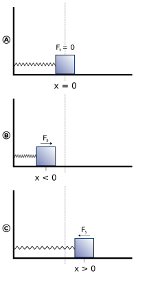
Spring–mass system in equilibrium (A), compressed (B) and stretched (C) states
When a spring is stretched or compressed by a mass, the spring develops a restoring force. Hooke's law gives the relationship of the force exerted by the spring when the spring is compressed or stretched a certain length:
where F is the force, k is the spring constant, and x is the displacement of the mass with respect to the equilibrium position. The minus sign in the equation indicates that the force exerted by the spring always acts in a direction that is opposite to the displacement (i.e. the force always acts towards the zero position), and so prevents the mass from flying off to infinity.
By using either force balance or an energy method, it can be readily shown that the motion of this system is given by the following differential equation:
If the initial displacement is A, and there is no initial velocity, the solution of this equation is given by
Given an ideal massless spring, is the mass on the end of the spring. If the spring itself has mass, its effective mass must be included in .
Energy variation in the spring–damping system
In terms of energy, all systems have two types of energy: potential energy and kinetic energy. When a spring is stretched or compressed, it stores elastic potential energy, which is then transferred into kinetic energy. The potential energy within a spring is determined by the equation
When the spring is stretched or compressed, kinetic energy of the mass gets converted into potential energy of the spring. By conservation of energy, assuming the datum is defined at the equilibrium position, when the spring reaches its maximal potential energy, the kinetic energy of the mass is zero. When the spring is released, it tries to return to equilibrium, and all its potential energy converts to kinetic energy of the mass.
In mechanics and physics, simple harmonic motion is a special type of periodic motion an object experiences due to a restoring force whose magnitude is directly proportional to the distance of the object from an equilibrium position and acts towards the equilibrium position. It results in an oscillation that is described by a sinusoid which continues indefinitely.
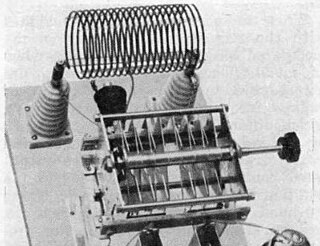
A phase-locked loop or phase lock loop (PLL) is a control system that generates an output signal whose phase is related to the phase of an input signal. There are several different types; the simplest is an electronic circuit consisting of a variable frequency oscillator and a phase detector in a feedback loop. The oscillator's frequency and phase are controlled proportionally by an applied voltage, hence the term voltage-controlled oscillator (VCO). The oscillator generates a periodic signal of a specific frequency, and the phase detector compares the phase of that signal with the phase of the input periodic signal, to adjust the oscillator to keep the phases matched.
Resonance is a phenomenon that occurs when an object or system is subjected to an external force or vibration that matches its natural frequency. When this happens, the object or system absorbs energy from the external force and starts vibrating with a larger amplitude. Resonance can occur in various systems, such as mechanical, electrical, or acoustic systems, and it is often desirable in certain applications, such as musical instruments or radio receivers. However, resonance can also be detrimental, leading to excessive vibrations or even structural failure in some cases.
The Navier–Stokes equations are partial differential equations which describe the motion of viscous fluid substances. They were named after French engineer and physicist Claude-Louis Navier and the Irish physicist and mathematician George Gabriel Stokes. They were developed over several decades of progressively building the theories, from 1822 (Navier) to 1842–1850 (Stokes).
In physics and engineering, the quality factor or Q factor is a dimensionless parameter that describes how underdamped an oscillator or resonator is. It is defined as the ratio of the initial energy stored in the resonator to the energy lost in one radian of the cycle of oscillation. Q factor is alternatively defined as the ratio of a resonator's centre frequency to its bandwidth when subject to an oscillating driving force. These two definitions give numerically similar, but not identical, results. Higher Q indicates a lower rate of energy loss and the oscillations die out more slowly. A pendulum suspended from a high-quality bearing, oscillating in air, has a high Q, while a pendulum immersed in oil has a low one. Resonators with high quality factors have low damping, so that they ring or vibrate longer.
In mathematics, theta functions are special functions of several complex variables. They show up in many topics, including Abelian varieties, moduli spaces, quadratic forms, and solitons. As Grassmann algebras, they appear in quantum field theory.
In general relativity, Schwarzschild geodesics describe the motion of test particles in the gravitational field of a central fixed mass that is, motion in the Schwarzschild metric. Schwarzschild geodesics have been pivotal in the validation of Einstein's theory of general relativity. For example, they provide accurate predictions of the anomalous precession of the planets in the Solar System and of the deflection of light by gravity.
Nondimensionalization is the partial or full removal of physical dimensions from an equation involving physical quantities by a suitable substitution of variables. This technique can simplify and parameterize problems where measured units are involved. It is closely related to dimensional analysis. In some physical systems, the term scaling is used interchangeably with nondimensionalization, in order to suggest that certain quantities are better measured relative to some appropriate unit. These units refer to quantities intrinsic to the system, rather than units such as SI units. Nondimensionalization is not the same as converting extensive quantities in an equation to intensive quantities, since the latter procedure results in variables that still carry units.
In physical systems, damping is the loss of energy of an oscillating system by dissipation. Damping is an influence within or upon an oscillatory system that has the effect of reducing or preventing its oscillation. Examples of damping include viscous damping in a fluid, surface friction, radiation, resistance in electronic oscillators, and absorption and scattering of light in optical oscillators. Damping not based on energy loss can be important in other oscillating systems such as those that occur in biological systems and bikes. Damping is not to be confused with friction, which is a type of dissipative force acting on a system. Friction can cause or be a factor of damping.
The Duffing equation, named after Georg Duffing (1861–1944), is a non-linear second-order differential equation used to model certain damped and driven oscillators. The equation is given by
Instantaneous phase and frequency are important concepts in signal processing that occur in the context of the representation and analysis of time-varying functions. The instantaneous phase (also known as local phase or simply phase) of a complex-valued function s(t), is the real-valued function:
In algebra, the Bring radical or ultraradical of a real number a is the unique real root of the polynomial
The Mason–Weaver equation describes the sedimentation and diffusion of solutes under a uniform force, usually a gravitational field. Assuming that the gravitational field is aligned in the z direction, the Mason–Weaver equation may be written
A parametric oscillator is a driven harmonic oscillator in which the oscillations are driven by varying some parameters of the system at some frequencies, typically different from the natural frequency of the oscillator. A simple example of a parametric oscillator is a child pumping a playground swing by periodically standing and squatting to increase the size of the swing's oscillations. The child's motions vary the moment of inertia of the swing as a pendulum. The "pump" motions of the child must be at twice the frequency of the swing's oscillations. Examples of parameters that may be varied are the oscillator's resonance frequency and damping .
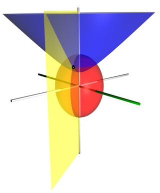
Toroidal coordinates are a three-dimensional orthogonal coordinate system that results from rotating the two-dimensional bipolar coordinate system about the axis that separates its two foci. Thus, the two foci and in bipolar coordinates become a ring of radius in the plane of the toroidal coordinate system; the -axis is the axis of rotation. The focal ring is also known as the reference circle.
Prolate spheroidal coordinates are a three-dimensional orthogonal coordinate system that results from rotating the two-dimensional elliptic coordinate system about the focal axis of the ellipse, i.e., the symmetry axis on which the foci are located. Rotation about the other axis produces oblate spheroidal coordinates. Prolate spheroidal coordinates can also be considered as a limiting case of ellipsoidal coordinates in which the two smallest principal axes are equal in length.
Oblate spheroidal coordinates are a three-dimensional orthogonal coordinate system that results from rotating the two-dimensional elliptic coordinate system about the non-focal axis of the ellipse, i.e., the symmetry axis that separates the foci. Thus, the two foci are transformed into a ring of radius in the x-y plane. Oblate spheroidal coordinates can also be considered as a limiting case of ellipsoidal coordinates in which the two largest semi-axes are equal in length.
In perturbation theory, the Poincaré–Lindstedt method or Lindstedt–Poincaré method is a technique for uniformly approximating periodic solutions to ordinary differential equations, when regular perturbation approaches fail. The method removes secular terms—terms growing without bound—arising in the straightforward application of perturbation theory to weakly nonlinear problems with finite oscillatory solutions.
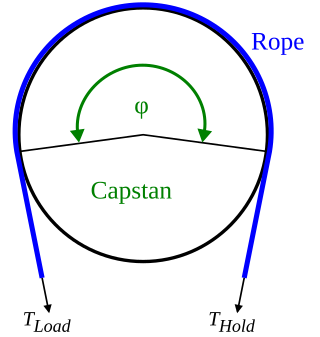
The capstan equation or belt friction equation, also known as Euler-Eytelwein formula, relates the hold-force to the load-force if a flexible line is wound around a cylinder.
An RLC circuit is an electrical circuit consisting of a resistor (R), an inductor (L), and a capacitor (C), connected in series or in parallel. The name of the circuit is derived from the letters that are used to denote the constituent components of this circuit, where the sequence of the components may vary from RLC.
This page is based on this Wikipedia article Text is available under the CC BY-SA 4.0 license; additional terms may apply. Images, videos and audio are available under their respective licenses.


![Step response of a damped harmonic oscillator; curves are plotted for three values of m = o1 = o0[?]1 - z. Time is in units of the decay time t = 1/(zo0). Step response for two-pole feedback amplifier.PNG](http://upload.wikimedia.org/wikipedia/commons/thumb/4/4f/Step_response_for_two-pole_feedback_amplifier.PNG/220px-Step_response_for_two-pole_feedback_amplifier.PNG)