In the physical science of dynamics, rigid-body dynamics studies the movement of systems of interconnected bodies under the action of external forces. The assumption that the bodies are rigid (i.e. they do not deform under the action of applied forces) simplifies analysis, by reducing the parameters that describe the configuration of the system to the translation and rotation of reference frames attached to each body.[1][2] This excludes bodies that display fluid, highly elastic, and plastic behavior.
The dynamics of a rigid body system is described by the laws of kinematics and by the application of Newton's second law (kinetics) or their derivative form, Lagrangian mechanics. The solution of these equations of motion provides a description of the position, the motion and the acceleration of the individual components of the system, and overall the system itself, as a function of time. The formulation and solution of rigid body dynamics is an important tool in the computer simulation of mechanical systems.
Planar rigid body dynamics
If a system of particles moves parallel to a fixed plane, the system is said to be constrained to planar movement. In this case, Newton's laws (kinetics) for a rigid system of N particles, Pi, i=1,...,N, simplify because there is no movement in the k direction. Determine the resultant force and torque at a reference point R, to obtain
where ri denotes the planar trajectory of each particle.
The kinematics of a rigid body yields the formula for the acceleration of the particle Pi in terms of the position R and acceleration A of the reference particle as well as the angular velocity vector ω and angular acceleration vector α of the rigid system of particles as,
For systems that are constrained to planar movement, the angular velocity and angular acceleration vectors are directed along k perpendicular to the plane of movement, which simplifies this acceleration equation. In this case, the acceleration vectors can be simplified by introducing the unit vectors ei from the reference point R to a point ri and the unit vectors , so
This yields the resultant force on the system as
and torque as
where and is the unit vector perpendicular to the plane for all of the particles Pi.
Use the center of massC as the reference point, so these equations for Newton's laws simplify to become
where M is the total mass and IC is the moment of inertia about an axis perpendicular to the movement of the rigid system and through the center of mass.
The first attempt to represent an orientation is attributed to Leonhard Euler. He imagined three reference frames that could rotate one around the other, and realized that by starting with a fixed reference frame and performing three rotations, he could get any other reference frame in the space (using two rotations to fix the vertical axis and another to fix the other two axes). The values of these three rotations are called Euler angles. Commonly, is used to denote precession, nutation, and intrinsic rotation.
Tait–Bryan angles, another way to describe orientation.
These are three angles, also known as yaw, pitch and roll, Navigation angles and Cardan angles. Mathematically they constitute a set of six possibilities inside the twelve possible sets of Euler angles, the ordering being the one best used for describing the orientation of a vehicle such as an airplane. In aerospace engineering they are usually referred to as Euler angles.
Euler also realized that the composition of two rotations is equivalent to a single rotation about a different fixed axis (Euler's rotation theorem). Therefore, the composition of the former three angles has to be equal to only one rotation, whose axis was complicated to calculate until matrices were developed.
Based on this fact he introduced a vectorial way to describe any rotation, with a vector on the rotation axis and module equal to the value of the angle. Therefore, any orientation can be represented by a rotation vector (also called Euler vector) that leads to it from the reference frame. When used to represent an orientation, the rotation vector is commonly called orientation vector, or attitude vector.
A similar method, called axis-angle representation, describes a rotation or orientation using a unit vector aligned with the rotation axis, and a separate value to indicate the angle (see figure).
With the introduction of matrices the Euler theorems were rewritten. The rotations were described by orthogonal matrices referred to as rotation matrices or direction cosine matrices. When used to represent an orientation, a rotation matrix is commonly called orientation matrix, or attitude matrix.
The above-mentioned Euler vector is the eigenvector of a rotation matrix (a rotation matrix has a unique real eigenvalue). The product of two rotation matrices is the composition of rotations. Therefore, as before, the orientation can be given as the rotation from the initial frame to achieve the frame that we want to describe.
The configuration space of a non-symmetrical object in n-dimensional space is SO(n)×Rn. Orientation may be visualized by attaching a basis of tangent vectors to an object. The direction in which each vector points determines its orientation.
Another way to describe rotations is using rotation quaternions, also called versors. They are equivalent to rotation matrices and rotation vectors. With respect to rotation vectors, they can be more easily converted to and from matrices. When used to represent orientations, rotation quaternions are typically called orientation quaternions or attitude quaternions.
Newton's second law in three dimensions
To consider rigid body dynamics in three-dimensional space, Newton's second law must be extended to define the relationship between the movement of a rigid body and the system of forces and torques that act on it.
Newton formulated his second law for a particle as, "The change of motion of an object is proportional to the force impressed and is made in the direction of the straight line in which the force is impressed."[3] Because Newton generally referred to mass times velocity as the "motion" of a particle, the phrase "change of motion" refers to the mass times acceleration of the particle, and so this law is usually written as
where F is understood to be the only external force acting on the particle, m is the mass of the particle, and a is its acceleration vector. The extension of Newton's second law to rigid bodies is achieved by considering a rigid system of particles.
Rigid system of particles
If a system of N particles, Pi, i=1,...,N, are assembled into a rigid body, then Newton's second law can be applied to each of the particles in the body. If Fi is the external force applied to particle Pi with mass mi, then
where Fij is the internal force of particle Pj acting on particle Pi that maintains the constant distance between these particles.
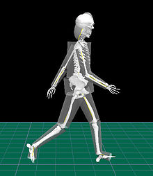
Human body modelled as a system of rigid bodies of geometrical solids. Representative bones were added for better visualization of the walking person.
An important simplification to these force equations is obtained by introducing the resultant force and torque that acts on the rigid system. This resultant force and torque is obtained by choosing one of the particles in the system as a reference point, R, where each of the external forces are applied with the addition of an associated torque. The resultant force F and torque T are given by the formulas,
where Ri is the vector that defines the position of particle Pi.
Newton's second law for a particle combines with these formulas for the resultant force and torque to yield,
where the internal forces Fij cancel in pairs. The kinematics of a rigid body yields the formula for the acceleration of the particle Pi in terms of the position R and acceleration a of the reference particle as well as the angular velocity vector ω and angular acceleration vector α of the rigid system of particles as,
Mass properties
The mass properties of the rigid body are represented by its center of mass and inertia matrix. Choose the reference point R so that it satisfies the condition
then it is known as the center of mass of the system.
The inertia matrix [IR] of the system relative to the reference point R is defined by
where is the column vector Ri − R; is its transpose, and is the 3 by 3 identity matrix.
is the scalar product of with itself, while is the tensor product of with itself.
Force-torque equations
Using the center of mass and inertia matrix, the force and torque equations for a single rigid body take the form
and are known as Newton's second law of motion for a rigid body.
The dynamics of an interconnected system of rigid bodies, Bi, j = 1, ..., M, is formulated by isolating each rigid body and introducing the interaction forces. The resultant of the external and interaction forces on each body, yields the force-torque equations
Newton's formulation yields 6M equations that define the dynamics of a system of M rigid bodies.[4]
Rotation in three dimensions
A rotating object, whether under the influence of torques or not, may exhibit the behaviours of precession and nutation. The fundamental equation describing the behavior of a rotating solid body is Euler's equation of motion:
where the pseudovectorsτ and L are, respectively, the torques on the body and its angular momentum, the scalar I is its moment of inertia, the vector ω is its angular velocity, the vector α is its angular acceleration, D is the differential in an inertial reference frame and d is the differential in a relative reference frame fixed with the body.
It follows from Euler's equation that a torque τ applied perpendicular to the axis of rotation, and therefore perpendicular to L, results in a rotation about an axis perpendicular to both τ and L. This motion is called precession. The angular velocity of precession ΩP is given by the cross product:[citation needed]
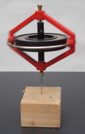
Precession can be demonstrated by placing a spinning top with its axis horizontal and supported loosely (frictionless toward precession) at one end. Instead of falling, as might be expected, the top appears to defy gravity by remaining with its axis horizontal, when the other end of the axis is left unsupported and the free end of the axis slowly describes a circle in a horizontal plane, the resulting precession turning. This effect is explained by the above equations. The torque on the top is supplied by a couple of forces: gravity acting downward on the device's centre of mass, and an equal force acting upward to support one end of the device. The rotation resulting from this torque is not downward, as might be intuitively expected, causing the device to fall, but perpendicular to both the gravitational torque (horizontal and perpendicular to the axis of rotation) and the axis of rotation (horizontal and outwards from the point of support), i.e., about a vertical axis, causing the device to rotate slowly about the supporting point.
Under a constant torque of magnitude τ, the speed of precession ΩP is inversely proportional to L, the magnitude of its angular momentum:
where θ is the angle between the vectors ΩP and L. Thus, if the top's spin slows down (for example, due to friction), its angular momentum decreases and so the rate of precession increases. This continues until the device is unable to rotate fast enough to support its own weight, when it stops precessing and falls off its support, mostly because friction against precession cause another precession that goes to cause the fall.
By convention, these three vectors - torque, spin, and precession - are all oriented with respect to each other according to the right-hand rule.
Virtual work of forces acting on a rigid body
An alternate formulation of rigid body dynamics that has a number of convenient features is obtained by considering the virtual work of forces acting on a rigid body.
The virtual work of forces acting at various points on a single rigid body can be calculated using the velocities of their point of application and the resultant force and torque. To see this, let the forces F1, F2 ... Fn act on the points R1, R2 ... Rn in a rigid body.
The trajectories of Ri, i = 1, ..., n are defined by the movement of the rigid body. The velocity of the points Ri along their trajectories are
where ω is the angular velocity vector of the body.
Virtual work
Work is computed from the dot product of each force with the displacement of its point of contact
If the trajectory of a rigid body is defined by a set of generalized coordinatesqj, j = 1, ..., m, then the virtual displacements δri are given by
The virtual work of this system of forces acting on the body in terms of the generalized coordinates becomes
or collecting the coefficients of δqj
Generalized forces
For simplicity consider a trajectory of a rigid body that is specified by a single generalized coordinate q, such as a rotation angle, then the formula becomes
Introduce the resultant force F and torque T so this equation takes the form
The quantity Q defined by
is known as the generalized force associated with the virtual displacement δq. This formula generalizes to the movement of a rigid body defined by more than one generalized coordinate, that is
where
It is useful to note that conservative forces such as gravity and spring forces are derivable from a potential function V(q1, ..., qn), known as a potential energy. In this case the generalized forces are given by
D'Alembert's form of the principle of virtual work
The equations of motion for a mechanical system of rigid bodies can be determined using D'Alembert's form of the principle of virtual work. The principle of virtual work is used to study the static equilibrium of a system of rigid bodies, however by introducing acceleration terms in Newton's laws this approach is generalized to define dynamic equilibrium.
Static equilibrium
The static equilibrium of a mechanical system rigid bodies is defined by the condition that the virtual work of the applied forces is zero for any virtual displacement of the system. This is known as the principle of virtual work.[5] This is equivalent to the requirement that the generalized forces for any virtual displacement are zero, that is Qi=0.
Let a mechanical system be constructed from n rigid bodies, Bi, i = 1, ..., n, and let the resultant of the applied forces on each body be the force-torque pairs, Fi and Ti, i = 1, ..., n. Notice that these applied forces do not include the reaction forces where the bodies are connected. Finally, assume that the velocity Vi and angular velocities ωi, i = 1, ..., n, for each rigid body, are defined by a single generalized coordinate q. Such a system of rigid bodies is said to have one degree of freedom.
The virtual work of the forces and torques, Fi and Ti, applied to this one degree of freedom system is given by
where
is the generalized force acting on this one degree of freedom system.
If the mechanical system is defined by m generalized coordinates, qj, j = 1, ..., m, then the system has m degrees of freedom and the virtual work is given by,
where
is the generalized force associated with the generalized coordinate qj. The principle of virtual work states that static equilibrium occurs when these generalized forces acting on the system are zero, that is
These m equations define the static equilibrium of the system of rigid bodies.
Generalized inertia forces
Consider a single rigid body which moves under the action of a resultant force F and torque T, with one degree of freedom defined by the generalized coordinate q. Assume the reference point for the resultant force and torque is the center of mass of the body, then the generalized inertia force Q* associated with the generalized coordinate q is given by
This inertia force can be computed from the kinetic energy of the rigid body,
by using the formula
A system of n rigid bodies with m generalized coordinates has the kinetic energy
which can be used to calculate the m generalized inertia forces[6]
Dynamic equilibrium
D'Alembert's form of the principle of virtual work states that a system of rigid bodies is in dynamic equilibrium when the virtual work of the sum of the applied forces and the inertial forces is zero for any virtual displacement of the system. Thus, dynamic equilibrium of a system of n rigid bodies with m generalized coordinates requires that
for any set of virtual displacements δqj. This condition yields m equations,
which can also be written as
The result is a set of m equations of motion that define the dynamics of the rigid body system.
Lagrange's equations
If the generalized forces Qj are derivable from a potential energy V(q1, ..., qm), then these equations of motion take the form
In this case, introduce the Lagrangian, L = T − V, so these equations of motion become
The linear and angular momentum of a rigid system of particles is formulated by measuring the position and velocity of the particles relative to the center of mass. Let the system of particles Pi, i = 1, ..., n be located at the coordinates ri and velocities vi. Select a reference point R and compute the relative position and velocity vectors,
The total linear and angular momentum vectors relative to the reference point R are
and
If R is chosen as the center of mass these equations simplify to
Rigid system of particles
To specialize these formulas to a rigid body, assume the particles are rigidly connected to each other so Pi, i=1,...,n are located by the coordinates ri and velocities vi. Select a reference point R and compute the relative position and velocity vectors,
where ω is the angular velocity of the system.[7][8][9]
In physics, angular momentum is the rotational analog of linear momentum. It is an important physical quantity because it is a conserved quantity – the total angular momentum of a closed system remains constant. Angular momentum has both a direction and a magnitude, and both are conserved. Bicycles and motorcycles, flying discs, rifled bullets, and gyroscopes owe their useful properties to conservation of angular momentum. Conservation of angular momentum is also why hurricanes form spirals and neutron stars have high rotational rates. In general, conservation limits the possible motion of a system, but it does not uniquely determine it.
Continuum mechanics is a branch of mechanics that deals with the deformation of and transmission of forces through materials modeled as a continuous mass rather than as discrete particles. The French mathematician Augustin-Louis Cauchy was the first to formulate such models in the 19th century.
In physics and mechanics, torque is the rotational analogue of linear force. It is also referred to as the moment of force. It describes the rate of change of angular momentum that would be imparted to an isolated body.
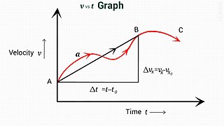
In physics, equations of motion are equations that describe the behavior of a physical system in terms of its motion as a function of time. More specifically, the equations of motion describe the behavior of a physical system as a set of mathematical functions in terms of dynamic variables. These variables are usually spatial coordinates and time, but may include momentum components. The most general choice are generalized coordinates which can be any convenient variables characteristic of the physical system. The functions are defined in a Euclidean space in classical mechanics, but are replaced by curved spaces in relativity. If the dynamics of a system is known, the equations are the solutions for the differential equations describing the motion of the dynamics.
Kinematics is a subfield of physics, developed in classical mechanics, that describes the motion of points, bodies (objects), and systems of bodies without considering the forces that cause them to move. Kinematics, as a field of study, is often referred to as the "geometry of motion" and is occasionally seen as a branch of mathematics. A kinematics problem begins by describing the geometry of the system and declaring the initial conditions of any known values of position, velocity and/or acceleration of points within the system. Then, using arguments from geometry, the position, velocity and acceleration of any unknown parts of the system can be determined. The study of how forces act on bodies falls within kinetics, not kinematics. For further details, see analytical dynamics.
In physics, angular acceleration is the time rate of change of angular velocity. Following the two types of angular velocity, spin angular velocity and orbital angular velocity, the respective types of angular acceleration are: spin angular acceleration, involving a rigid body about an axis of rotation intersecting the body's centroid; and orbital angular acceleration, involving a point particle and an external axis.
In physics, work is the energy transferred to or from an object via the application of force along a displacement. In its simplest form, for a constant force aligned with the direction of motion, the work equals the product of the force strength and the distance traveled. A force is said to do positive work if when applied it has a component in the direction of the displacement of the point of application. A force does negative work if it has a component opposite to the direction of the displacement at the point of application of the force.
The moment of inertia, otherwise known as the mass moment of inertia, angular mass, second moment of mass, or most accurately, rotational inertia, of a rigid body is a quantity that determines the torque needed for a desired angular acceleration about a rotational axis, akin to how mass determines the force needed for a desired acceleration. It depends on the body's mass distribution and the axis chosen, with larger moments requiring more torque to change the body's rate of rotation.
The vorticity equation of fluid dynamics describes the evolution of the vorticity ω of a particle of a fluid as it moves with its flow; that is, the local rotation of the fluid. The governing equation is:
In classical mechanics, Euler's rotation equations are a vectorial quasilinear first-order ordinary differential equation describing the rotation of a rigid body, using a rotating reference frame with angular velocity ω whose axes are fixed to the body. Their general vector form is
In mechanics, virtual work arises in the application of the principle of least action to the study of forces and movement of a mechanical system. The work of a force acting on a particle as it moves along a displacement is different for different displacements. Among all the possible displacements that a particle may follow, called virtual displacements, one will minimize the action. This displacement is therefore the displacement followed by the particle according to the principle of least action.
The work of a force on a particle along a virtual displacement is known as the virtual work.
Screw theory is the algebraic calculation of pairs of vectors, such as forces and moments or angular and linear velocity, that arise in the kinematics and dynamics of rigid bodies. The mathematical framework was developed by Sir Robert Stawell Ball in 1876 for application in kinematics and statics of mechanisms.
In differential geometry, the four-gradient is the four-vector analogue of the gradient from vector calculus.
In geometry and linear algebra, a Cartesian tensor uses an orthonormal basis to represent a tensor in a Euclidean space in the form of components. Converting a tensor's components from one such basis to another is done through an orthogonal transformation.
Stokes flow, also named creeping flow or creeping motion, is a type of fluid flow where advective inertial forces are small compared with viscous forces. The Reynolds number is low, i.e. . This is a typical situation in flows where the fluid velocities are very slow, the viscosities are very large, or the length-scales of the flow are very small. Creeping flow was first studied to understand lubrication. In nature, this type of flow occurs in the swimming of microorganisms and sperm. In technology, it occurs in paint, MEMS devices, and in the flow of viscous polymers generally.
In continuum mechanics, the finite strain theory—also called large strain theory, or large deformation theory—deals with deformations in which strains and/or rotations are large enough to invalidate assumptions inherent in infinitesimal strain theory. In this case, the undeformed and deformed configurations of the continuum are significantly different, requiring a clear distinction between them. This is commonly the case with elastomers, plastically-deforming materials and other fluids and biological soft tissue.
Rotation around a fixed axis or axial rotation is a special case of rotational motion around a axis of rotation fixed, stationary, or static in three-dimensional space. This type of motion excludes the possibility of the instantaneous axis of rotation changing its orientation and cannot describe such phenomena as wobbling or precession. According to Euler's rotation theorem, simultaneous rotation along a number of stationary axes at the same time is impossible; if two rotations are forced at the same time, a new axis of rotation will result.
In classical mechanics, Appell's equation of motion is an alternative general formulation of classical mechanics described by Josiah Willard Gibbs in 1879 and Paul Émile Appell in 1900.
In physics, relativistic angular momentum refers to the mathematical formalisms and physical concepts that define angular momentum in special relativity (SR) and general relativity (GR). The relativistic quantity is subtly different from the three-dimensional quantity in classical mechanics.
References
↑ B. Paul, Kinematics and Dynamics of Planar Machinery, Prentice-Hall, NJ, 1979
↑ L. W. Tsai, Robot Analysis: The mechanics of serial and parallel manipulators, John-Wiley, NY, 1999.
↑ Torby, Bruce (1984). "Energy Methods". Advanced Dynamics for Engineers. HRW Series in Mechanical Engineering. United States of America: CBS College Publishing. ISBN0-03-063366-4.
This page is based on this Wikipedia article Text is available under the CC BY-SA 4.0 license; additional terms may apply. Images, videos and audio are available under their respective licenses.